4.3. PySpark#
4.3.1. Spark Environment#
4.3.1.1. Cơ chế hoạt động của spark#
Bước đầu tiên để thiết lập spark là tạo ra 1 cụm xử lý (cluster) trên một máy chủ. Cụm xử lý này được kết nối tới rất nhiều nodes khác nhau. Máy chủ (master) sẽ làm nhiệm vụ: phân chia dữ liệu và quản lý tính toán trên các máy con. máy chủ sẽ kết nối đến các máy con (slaves) trong cụm bằng các session. Máy chủ sẽ gửi dữ liệu và yêu cầu tính toán để máy con thực thi. Sau khi có kết quả máy con có nhiệm vụ trả về máy chủ. Máy chủ tổng hợp tất cả các tính toán trên máy con để tính ra kết quả cuối cùng.
Trong bài này do mới làm quen với spark nên mình sẽ khởi tạo một cluster trên local. Thay vì kết nối tới những máy khác, các tính toán sẽ được thực hiện chỉ trên server local thông qua một giả lập cụm.
Để kiểm tra các schema có trong một table chúng ta sử dụng hàm printSchema()
4.3.1.2. Khởi tạo môi trường spark#
Để khởi tạo một connection chúng ta đơn giản là tạo ra một instance của SparkContext class. Class này sẽ có một vài tham số yêu cầu chúng ta phải khai báo để xác định các thuộc tính của cụm mà chúng ta muốn connect tới.
Những tham số này có thể được cấu hình thông qua constructor SparkConf().
Một vài tham số quan trọng:
Master: url connect tới master.AppName: Tên ứng dụng.SparkHome: Đường dẫn nơi spark được cài đặt trên các nodes.
from pyspark import SparkContext

# Stop spark if it existed.
try:
    sc.stop()
except:
    print("sc have not yet created!")

sc = SparkContext(master="local", appName="First app")
# Check spark context
print(sc)
# Check spark context version
print(sc.version)
sc have not yet created!
<SparkContext master=local appName=First app>
3.5.2
Lưu ý chúng ta chỉ có thể khởi tạo
SparkContext1 lần nên nếu chưa stop sc mà chạy lại lệnh trên sẽ bị lỗi. Do đó lệnhSparkContext.getOrCreate()được sử dụng để khởi tạo mớiSparkContextnếu nó chưa xuất hiện và lấy lạiSparkContextcũ nếu đã được khởi tạo và đang run.
4.3.1.3. Tìm kiếm spark environment#
# find the env spark
import findspark

findspark.init()

import pyspark

# khởi tạo trình chạy pyspark
from pyspark.sql import SparkSession

spark = SparkSession.builder.appName("Lesson1").getOrCreate()
spark
SparkSession - in-memory
# check cores
spark._jsc.sc().getExecutorMemoryStatus().keySet().size()
1
4.3.1.4. Khởi tạo section#
Như vậy sau bước trên ta đã có môi trường kết nối tới cluster. Tuy nhiên để hoạt động được trong môi trường này thì chúng ta cần phải khởi tạo session thông qua hàm SparkSession.
from pyspark.sql import SparkSession

my_spark = SparkSession.builder.getOrCreate()
# Print my_spark session
print(my_spark)
<pyspark.sql.session.SparkSession object at 0x105383c90>
Hàm
getOrCreate()của session cũng tương tự như context để tránh trường hợp phát sinh lỗi khi session đã tồn tại và đang hoạt động nhưng được khởi tạo lại.
4.3.2. DataFrame Creation#
# List all table exist in spark sesion
my_spark.catalog.listTables()
[]
4.3.2.1. Import dataframe to catelog#
Tuy nhiên lúc này flights vẫn chỉ là một spark DataFrame chưa có trong catalog của của cluster. Sử dụng hàm listTable() liệt kê danh sách bảng ta thu được 1 list rỗng.
Lý do là bởi khi được đọc từ hàm read.csv() thì dữ liệu chỉ được lưu trữ ở Local dưới dạng một spark DataFrame. Để đưa dự liệu từ local lên cluster chúng ta cần save nó dưới dạng một temporary table thông một trong những lệnh bên dưới:
.createTempView(): là một phương thức của spark DataFrame trong đó tham số duy nhất được truyền vào là tên bảng mà bạn muốn lưu trữ dưới dạng temporary table. Bảng được tạo ra là tạm thời và chỉ có thể được truy cập từ session được sử dụng để tạo ra spark DataFrame..createOrReplaceTempView(): Có tác dụng hoàn toàn giống như .createTempView() nhưng nó sẽ update lại temporary table nếu nó đã tồn tại hoặc tạo mới nếu chưa tồn tại trước dây. Tránh trường hợp duplicate dữ liệu..createDataFrame(): Tạo một spark DataFrame từ một pandas DataFrame.
Để hiểu rõ hơn về nguyên tắc khởi tạo bảng chúng ta có thể xem sơ đồ bên dưới:

Spark Cluster sẽ tương tác với user thông qua kết nối từ SparkContext. Có 2 dạng lưu trữ chính ở SparkContext là spark DataFrame và catalog. Trong đó spark DataFrame là định dạng dạng bảng được lưu trữ ở Local và catalog là các temporary table sống trong các SparkSession. Để dữ liệu có thể truy cập từ một session chúng ta cần chuyển nó từ định dạng spark DataFrame sang temporary table thông qua hàm .createTempView() hoặc .createOrReplaceTempView().
Bên dưới ta sẽ khởi tạo một temporary table với tên là flights_temp cho bảng flights.
# Create a temporary table on catalog of local data frame flights as new temporary table flights_temp on catalog
flights.createOrReplaceTempView("flights_temp")
# check list all table available on catalog
my_spark.catalog.listTables()
[Table(name='flights_temp', catalog=None, namespace=[], description=None, tableType='TEMPORARY', isTemporary=True)]
4.3.2.2. Create dataframe#
# create from row
from datetime import datetime, date
import pandas as pd
from pyspark.sql import Row

df = spark.createDataFrame(
    [
        Row(
            a=1,
            b=2.0,
            c="string1",
            d=date(2000, 1, 1),
            e=datetime(2000, 1, 1, 12, 0),
        ),
        Row(
            a=2,
            b=3.0,
            c="string2",
            d=date(2000, 2, 1),
            e=datetime(2000, 1, 2, 12, 0),
        ),
        Row(
            a=4,
            b=5.0,
            c="string3",
            d=date(2000, 3, 1),
            e=datetime(2000, 1, 3, 12, 0),
        ),
    ]
)
df.show()
+---+---+-------+----------+-------------------+
|  a|  b|      c|         d|                  e|
+---+---+-------+----------+-------------------+
|  1|2.0|string1|2000-01-01|2000-01-01 12:00:00|
|  2|3.0|string2|2000-02-01|2000-01-02 12:00:00|
|  4|5.0|string3|2000-03-01|2000-01-03 12:00:00|
+---+---+-------+----------+-------------------+
# create from tuple
df = spark.createDataFrame(
    [
        (1, 2.0, "string1", date(2000, 1, 1), datetime(2000, 1, 1, 12, 0)),
        (2, 3.0, "string2", date(2000, 2, 1), datetime(2000, 1, 2, 12, 0)),
        (3, 4.0, "string3", date(2000, 3, 1), datetime(2000, 1, 3, 12, 0)),
    ],
    schema="a long, b double, c string, d date, e timestamp",
)
df
DataFrame[a: bigint, b: double, c: string, d: date, e: timestamp]
# Create a PySpark DataFrame from an RDD consisting of a list of tuples.
rdd = spark.sparkContext.parallelize(
    [
        (1, 2.0, "string1", date(2000, 1, 1), datetime(2000, 1, 1, 12, 0)),
        (2, 3.0, "string2", date(2000, 2, 1), datetime(2000, 1, 2, 12, 0)),
        (3, 4.0, "string3", date(2000, 3, 1), datetime(2000, 1, 3, 12, 0)),
    ]
)
df = spark.createDataFrame(rdd, schema=["a", "b", "c", "d", "e"])
df
DataFrame[a: bigint, b: double, c: string, d: date, e: timestamp]
# from pandas.dataframe
pandas_df = pd.DataFrame(
    {
        "a": [1, 2, 3],
        "b": [2.0, 3.0, 4.0],
        "c": ["string1", "string2", "string3"],
        "d": [date(2000, 1, 1), date(2000, 2, 1), date(2000, 3, 1)],
        "e": [
            datetime(2000, 1, 1, 12, 0),
            datetime(2000, 1, 2, 12, 0),
            datetime(2000, 1, 3, 12, 0),
        ],
    }
)
df = spark.createDataFrame(pandas_df)
df
DataFrame[a: bigint, b: double, c: string, d: date, e: timestamp]
4.3.2.3. Reading file#
import os

file = os.path.normpath(
    os.path.join(os.getcwd(), "..", "0. Data", "datatest.csv")
)  ## ".." to get out folder
file
'J:\\My Drive\\GitCode\\My_learning\\11. BigData\\0. Data\\datatest.csv'
df = spark.read.csv(file, header=True)
df.show(1)
+---+------------+-----------+------------+-----------+-------+
|_c0|sepal_length|sepal_width|petal_length|petal_width|species|
+---+------------+-----------+------------+-----------+-------+
|  0|         5.1|        3.5|         1.4|        0.2| setosa|
+---+------------+-----------+------------+-----------+-------+
only showing top 1 row
# csv
import os

# file = os.path.normpath(os.path.join(os.getcwd(),"..","2.Dask",'datatest','1989.csv')) ## ".." to get out folder
df = spark.read.csv(
    r"J:\My Drive\GitCode\My_learning\11. BigData\0. Data\datatest.csv",
    header=True,
)
df.show(1)
+---+------------+-----------+------------+-----------+-------+
|_c0|sepal_length|sepal_width|petal_length|petal_width|species|
+---+------------+-----------+------------+-----------+-------+
|  0|         5.1|        3.5|         1.4|        0.2| setosa|
+---+------------+-----------+------------+-----------+-------+
only showing top 1 row
import myfunction as mf

mf.display(df.limit(4).toPandas())
| _c0 | sepal_length | sepal_width | petal_length | petal_width | species | |
|---|---|---|---|---|---|---|
| 0 | 0 | 5.1 | 3.5 | 1.4 | 0.2 | setosa |
| 1 | 1 | 4.9 | 3.0 | 1.4 | 0.2 | setosa |
| 2 | 2 | 4.7 | 3.2 | 1.3 | 0.2 | setosa |
| 3 | 3 | 4.6 | 3.1 | 1.5 | 0.2 | setosa |
# read parquet
df = spark.read.parquet("data.parquet")  # read file parquet

# read many file parquet with the sample form
df_all = spark.read.parquet("data*.parquet")
df1_2 = spark.read.parquet("data1.parquet", "data2.parquet")
df = spark.read.option("bathPath", path).parquet(
    path + "//data*.parquet"
)  # set option
df = spark.read.parquet(
    folder1 + "//data*.parquet", folder2 + "//*"
)  # set option
4.3.3. Dataframe function#
4.3.3.1. Viewing#
df.limit(3).show()
+---+------------+-----------+------------+-----------+-------+
|_c0|sepal_length|sepal_width|petal_length|petal_width|species|
+---+------------+-----------+------------+-----------+-------+
|  0|         5.1|        3.5|         1.4|        0.2| setosa|
|  1|         4.9|        3.0|         1.4|        0.2| setosa|
|  2|         4.7|        3.2|         1.3|        0.2| setosa|
+---+------------+-----------+------------+-----------+-------+
# show sample
df.show(1)
+---+---+-------+----------+-------------------+
|  a|  b|      c|         d|                  e|
+---+---+-------+----------+-------------------+
|  1|2.0|string1|2000-01-01|2000-01-01 12:00:00|
+---+---+-------+----------+-------------------+
only showing top 1 row
df.show(1, vertical=True)
-RECORD 0------------------
 a   | 1
 b   | 2.0
 c   | string1
 d   | 2000-01-01
 e   | 2000-01-01 12:00:00
only showing top 1 row
# len df
df.count()
3
spark.sql.repl.eagerEval.maxNumRows  # setup maxrow to show
spark.conf.set(
    "spark.sql.repl.eagerEval.enabled", True
)  # setup config to show in jupyter
df
| a | b | c | d | e |
|---|---|---|---|---|
| 1 | 2.0 | string1 | 2000-01-01 | 2000-01-01 12:00:00 |
| 2 | 3.0 | string2 | 2000-02-01 | 2000-01-02 12:00:00 |
| 3 | 4.0 | string3 | 2000-03-01 | 2000-01-03 12:00:00 |
# dtype
df.printSchema()
root
 |-- a: long (nullable = true)
 |-- b: double (nullable = true)
 |-- c: string (nullable = true)
 |-- d: date (nullable = true)
 |-- e: timestamp (nullable = true)
# convert pandas.df
df.toPandas()
| a | b | c | d | e | |
|---|---|---|---|---|---|
| 0 | 1 | 2.0 | string1 | 2000-01-01 | 2000-01-01 12:00:00 |
| 1 | 2 | 3.0 | string2 | 2000-02-01 | 2000-01-02 12:00:00 |
| 2 | 3 | 4.0 | string3 | 2000-03-01 | 2000-01-03 12:00:00 |
# show columns
df.columns
['a', 'b', 'c', 'd', 'e']
4.3.3.2. Validate datatype#
df.printSchema() # get dtype by SAMPLE of beginning datafile
root
 |-- _c0: string (nullable = true)
 |-- sepal_length: string (nullable = true)
 |-- sepal_width: string (nullable = true)
 |-- petal_length: string (nullable = true)
 |-- petal_width: string (nullable = true)
 |-- species: string (nullable = true)
df.describe()
DataFrame[summary: string, _c0: string, sepal_length: string, sepal_width: string, petal_length: string, petal_width: string, species: string]
df.schema["sepal_length"]
StructField('sepal_length', StringType(), True)
from pyspark.sql.types import *

# set schema
data_schema = [
    # StructField('_c0',IntegerType()),
    StructField("sepal_length", FloatType()),
    StructField("sepal_width", FloatType()),
    # StructField('petal_length',FloatType()), # dont need to set all
    StructField("petal_width", FloatType()),
    StructField("species", StringType()),
]

final_struc = StructType(fields=data_schema)

df = spark.read.csv(file, header=True, schema=final_struc)

df.printSchema()  # chỉ đọc những cột có định nghĩa trong final_struc schema
root
 |-- sepal_length: float (nullable = true)
 |-- sepal_width: float (nullable = true)
 |-- petal_width: float (nullable = true)
 |-- species: string (nullable = true)
df.show(2)
df.printSchema()
+---+------------+-----------+------------+-----------+-------+
|_c0|sepal_length|sepal_width|petal_length|petal_width|species|
+---+------------+-----------+------------+-----------+-------+
|  0|         5.1|        3.5|         1.4|        0.2| setosa|
|  1|         4.9|        3.0|         1.4|        0.2| setosa|
+---+------------+-----------+------------+-----------+-------+
only showing top 2 rows

root
 |-- _c0: string (nullable = true)
 |-- sepal_length: string (nullable = true)
 |-- sepal_width: string (nullable = true)
 |-- petal_length: string (nullable = true)
 |-- petal_width: string (nullable = true)
 |-- species: string (nullable = true)
# change the dtype columns
from pyspark.sql.types import *

df = (
    df.withColumn("sepal_length", df["sepal_length"].cast(FloatType()))
    .withColumn("sepal_width", df["sepal_width"].cast(IntegerType()))
    .withColumn("sepal_length", to_date(df["sepal_length"], "yy.dd.mm"))
    .withColumn("sepal_length", to_timestamp(df["petal_width"], "yy.dd.mm"))
)
4.3.3.3. Thêm một trường mới vào một bảng sẵn có#
.withColumn(“newColumnName”, formular)
Gồm 2 tham số chính, tham số thứ nhất là tên trường mới, tham số thứ 2 là công thức cập nhật tên trường.
# thêm 1 trường mới là HOUR_ARR được tính dựa trên AIR_TIME/60 (qui từ phút ra h) của bảng flights
flights = flights.withColumn("HOUR_ARR", flights.AIR_TIME / 60)
Lưu ý rằng spark DataFrame là một dạng dữ liệu immutable (không thể modified được). Do đó ta không thể inplace update (như các hàm fillna() hoặc replace() của pandas dataframe) mà cần phải gán giá trị trả về vào chính tên bảng ban đầu để cập nhật trường mới.
flights.show(3)
+----+-----+---+-----------+-------+-------------+-----------+--------------+-------------------+-------------------+--------------+---------------+--------+----------+--------------+------------+--------+--------+---------+-------+-----------------+------------+-------------+--------+---------+-------------------+----------------+--------------+-------------+-------------------+-------------+-----------------+
|YEAR|MONTH|DAY|DAY_OF_WEEK|AIRLINE|FLIGHT_NUMBER|TAIL_NUMBER|ORIGIN_AIRPORT|DESTINATION_AIRPORT|SCHEDULED_DEPARTURE|DEPARTURE_TIME|DEPARTURE_DELAY|TAXI_OUT|WHEELS_OFF|SCHEDULED_TIME|ELAPSED_TIME|AIR_TIME|DISTANCE|WHEELS_ON|TAXI_IN|SCHEDULED_ARRIVAL|ARRIVAL_TIME|ARRIVAL_DELAY|DIVERTED|CANCELLED|CANCELLATION_REASON|AIR_SYSTEM_DELAY|SECURITY_DELAY|AIRLINE_DELAY|LATE_AIRCRAFT_DELAY|WEATHER_DELAY|         HOUR_ARR|
+----+-----+---+-----------+-------+-------------+-----------+--------------+-------------------+-------------------+--------------+---------------+--------+----------+--------------+------------+--------+--------+---------+-------+-----------------+------------+-------------+--------+---------+-------------------+----------------+--------------+-------------+-------------------+-------------+-----------------+
|2015|    1|  1|          4|     AS|           98|     N407AS|           ANC|                SEA|               0005|          2354|            -11|      21|      0015|           205|         194|     169|    1448|     0404|      4|             0430|        0408|          -22|       0|        0|               NULL|            NULL|          NULL|         NULL|               NULL|         NULL|2.816666666666667|
|2015|    1|  1|          4|     AA|         2336|     N3KUAA|           LAX|                PBI|               0010|          0002|             -8|      12|      0014|           280|         279|     263|    2330|     0737|      4|             0750|        0741|           -9|       0|        0|               NULL|            NULL|          NULL|         NULL|               NULL|         NULL|4.383333333333334|
|2015|    1|  1|          4|     US|          840|     N171US|           SFO|                CLT|               0020|          0018|             -2|      16|      0034|           286|         293|     266|    2296|     0800|     11|             0806|        0811|            5|       0|        0|               NULL|            NULL|          NULL|         NULL|               NULL|         NULL|4.433333333333334|
+----+-----+---+-----------+-------+-------------+-----------+--------------+-------------------+-------------------+--------------+---------------+--------+----------+--------------+------------+--------+--------+---------+-------+-----------------+------------+-------------+--------+---------+-------------------+----------------+--------------+-------------+-------------------+-------------+-----------------+
only showing top 3 rows
4.3.3.4. Lựa chọn danh sách các trường#
.select(“column1”, “column2”, … , “columnt”, formular)
tên column được truyền vào đưới dạng string và tạo ra một trường mới thông qua formular
Lưu ý để đặt tên cho trường mới ứng với formular chúng ta sẽ cần sử dụng hàm
formula.alias("columnName")
# tạo ra trường avg_speed tính vận tốc trung bình của các máy bay bằng cách lấy khoảng cách (DISTANCE) chia cho thời gian bay (HOUR_ARR)
# group by theo mã máy bay (TAIL_NUMBER) bằng lệnh select

avg_speed = flights.select(
    "ORIGIN_AIRPORT",
    "DESTINATION_AIRPORT",
    "TAIL_NUMBER",
    (flights.DISTANCE / flights.HOUR_ARR).alias("avg_speed"),
)
avg_speed.printSchema()
avg_speed.show(5)
root
 |-- ORIGIN_AIRPORT: string (nullable = true)
 |-- DESTINATION_AIRPORT: string (nullable = true)
 |-- TAIL_NUMBER: string (nullable = true)
 |-- avg_speed: double (nullable = true)

+--------------+-------------------+-----------+-----------------+
|ORIGIN_AIRPORT|DESTINATION_AIRPORT|TAIL_NUMBER|        avg_speed|
+--------------+-------------------+-----------+-----------------+
|           ANC|                SEA|     N407AS|514.0828402366864|
|           LAX|                PBI|     N3KUAA|531.5589353612166|
|           SFO|                CLT|     N171US|517.8947368421052|
|           LAX|                MIA|     N3HYAA|544.6511627906978|
|           SEA|                ANC|     N527AS|436.5829145728643|
+--------------+-------------------+-----------+-----------------+
only showing top 5 rows
.selectExpr(“column1”, “column2”, … , “columnt”, “formularExpr”)
Hoàn toàn tương tự như .select() nhưng tham số formular được thay thế bằng chuỗi string biểu diễn công thức như trong câu lệnh SQL.
avg_speed_exp = flights.selectExpr(
    "ORIGIN_AIRPORT",
    "DESTINATION_AIRPORT",
    "TAIL_NUMBER",
    "(DISTANCE/HOUR_ARR) AS avg_speed",
)
avg_speed_exp.printSchema()
avg_speed_exp.show(5)
root
 |-- ORIGIN_AIRPORT: string (nullable = true)
 |-- DESTINATION_AIRPORT: string (nullable = true)
 |-- TAIL_NUMBER: string (nullable = true)
 |-- avg_speed: double (nullable = true)

+--------------+-------------------+-----------+-----------------+
|ORIGIN_AIRPORT|DESTINATION_AIRPORT|TAIL_NUMBER|        avg_speed|
+--------------+-------------------+-----------+-----------------+
|           ANC|                SEA|     N407AS|514.0828402366864|
|           LAX|                PBI|     N3KUAA|531.5589353612166|
|           SFO|                CLT|     N171US|517.8947368421052|
|           LAX|                MIA|     N3HYAA|544.6511627906978|
|           SEA|                ANC|     N527AS|436.5829145728643|
+--------------+-------------------+-----------+-----------------+
only showing top 5 rows
4.3.3.5. Đổi tên của một column name#
.withColumnRenamed(“oldColumnName”, “newColumnName”)
4.3.3.6. Đổi định dạng data cột#
.withColumn("conlumnName", value)
4.3.3.7. Filter bảng#
.filter(condition)
Condition có thể làm một string expression biểu diễn công thức lọc hoặc một công thức giữa các trường trong spark DataFrame.
Lưu ý Condition phải trả về một trường dạng Boolean type
filter_SEA_ANC = flights.filter("ORIGIN_AIRPORT == 'SEA'").filter(
    "DESTINATION_AIRPORT == 'ANC'"
)
filter_SEA_ANC.show(5)
+----+-----+---+-----------+-------+-------------+-----------+--------------+-------------------+-------------------+--------------+---------------+--------+----------+--------------+------------+--------+--------+---------+-------+-----------------+------------+-------------+--------+---------+-------------------+----------------+--------------+-------------+-------------------+-------------+------------------+
|YEAR|MONTH|DAY|DAY_OF_WEEK|AIRLINE|FLIGHT_NUMBER|TAIL_NUMBER|ORIGIN_AIRPORT|DESTINATION_AIRPORT|SCHEDULED_DEPARTURE|DEPARTURE_TIME|DEPARTURE_DELAY|TAXI_OUT|WHEELS_OFF|SCHEDULED_TIME|ELAPSED_TIME|AIR_TIME|DISTANCE|WHEELS_ON|TAXI_IN|SCHEDULED_ARRIVAL|ARRIVAL_TIME|ARRIVAL_DELAY|DIVERTED|CANCELLED|CANCELLATION_REASON|AIR_SYSTEM_DELAY|SECURITY_DELAY|AIRLINE_DELAY|LATE_AIRCRAFT_DELAY|WEATHER_DELAY|          HOUR_ARR|
+----+-----+---+-----------+-------+-------------+-----------+--------------+-------------------+-------------------+--------------+---------------+--------+----------+--------------+------------+--------+--------+---------+-------+-----------------+------------+-------------+--------+---------+-------------------+----------------+--------------+-------------+-------------------+-------------+------------------+
|2015|    1|  1|          4|     AS|          135|     N527AS|           SEA|                ANC|               0025|          0024|             -1|      11|      0035|           235|         215|     199|    1448|     0254|      5|             0320|        0259|          -21|       0|        0|               NULL|            NULL|          NULL|         NULL|               NULL|         NULL| 3.316666666666667|
|2015|    1|  1|          4|     AS|           81|     N577AS|           SEA|                ANC|               0600|          0557|             -3|      25|      0622|           234|         224|     195|    1448|     0837|      4|             0854|        0841|          -13|       0|        0|               NULL|            NULL|          NULL|         NULL|               NULL|         NULL|              3.25|
|2015|    1|  1|          4|     AS|           83|     N532AS|           SEA|                ANC|               0800|          0802|              2|      14|      0816|           235|         211|     194|    1448|     1030|      3|             1055|        1033|          -22|       0|        0|               NULL|            NULL|          NULL|         NULL|               NULL|         NULL|3.2333333333333334|
|2015|    1|  1|          4|     AS|          111|     N570AS|           SEA|                ANC|               0905|          0859|             -6|      30|      0929|           230|         226|     193|    1448|     1142|      3|             1155|        1145|          -10|       0|        0|               NULL|            NULL|          NULL|         NULL|               NULL|         NULL| 3.216666666666667|
|2015|    1|  1|          4|     AS|           85|     N764AS|           SEA|                ANC|               1020|          1020|              0|      19|      1039|           223|         220|     198|    1448|     1257|      3|             1303|        1300|           -3|       0|        0|               NULL|            NULL|          NULL|         NULL|               NULL|         NULL|               3.3|
+----+-----+---+-----------+-------+-------------+-----------+--------------+-------------------+-------------------+--------------+---------------+--------+----------+--------------+------------+--------+--------+---------+-------+-----------------+------------+-------------+--------+---------+-------------------+----------------+--------------+-------------+-------------------+-------------+------------------+
only showing top 5 rows
import os

# file = os.path.normpath(os.path.join(os.getcwd(),"..","2.Dask",'datatest','1989.csv')) ## ".." to get out folder
df = spark.read.csv(
    r"J:\My Drive\GitCode\My_learning\11. BigData\0. Data\datatest.csv",
    header=True,
)
df.show(1)
+---+------------+-----------+------------+-----------+-------+
|_c0|sepal_length|sepal_width|petal_length|petal_width|species|
+---+------------+-----------+------------+-----------+-------+
|  0|         5.1|        3.5|         1.4|        0.2| setosa|
+---+------------+-----------+------------+-----------+-------+
only showing top 1 row
# filter
df.filter(df.sepal_length == 5.1).show()
+---+------------+-----------+------------+-----------+----------+
|_c0|sepal_length|sepal_width|petal_length|petal_width|   species|
+---+------------+-----------+------------+-----------+----------+
|  0|         5.1|        3.5|         1.4|        0.2|    setosa|
| 17|         5.1|        3.5|         1.4|        0.3|    setosa|
| 19|         5.1|        3.8|         1.5|        0.3|    setosa|
| 21|         5.1|        3.7|         1.5|        0.4|    setosa|
| 23|         5.1|        3.3|         1.7|        0.5|    setosa|
| 39|         5.1|        3.4|         1.5|        0.2|    setosa|
| 44|         5.1|        3.8|         1.9|        0.4|    setosa|
| 46|         5.1|        3.8|         1.6|        0.2|    setosa|
| 98|         5.1|        2.5|         3.0|        1.1|versicolor|
+---+------------+-----------+------------+-----------+----------+
# where va filter la nhu nhau
df.select(["sepal_length", "sepal_width", "petal_length", "species"]).where(
    df.species.like("%eto%")
).show(2)
+------------+-----------+------------+-------+
|sepal_length|sepal_width|petal_length|species|
+------------+-----------+------------+-------+
|         5.1|        3.5|         1.4| setosa|
|         4.9|        3.0|         1.4| setosa|
+------------+-----------+------------+-------+
only showing top 2 rows
df.select("species", df.species.substr(-4, 3)).show(
    2
)  # string lấy substring từ -4, 3 ký tu
+-------+-------------------------+
|species|substring(species, -4, 3)|
+-------+-------------------------+
| setosa|                      tos|
| setosa|                      tos|
| setosa|                      tos|
+-------+-------------------------+
only showing top 3 rows
df[df.species.isin("setosa", "versicolor")].show(2)  # isin
df[df.species.startswith("s")].show(2)  # startswith
+---+------------+-----------+------------+-----------+-------+
|_c0|sepal_length|sepal_width|petal_length|petal_width|species|
+---+------------+-----------+------------+-----------+-------+
|  0|         5.1|        3.5|         1.4|        0.2| setosa|
|  1|         4.9|        3.0|         1.4|        0.2| setosa|
+---+------------+-----------+------------+-----------+-------+
only showing top 2 rows

+---+------------+-----------+------------+-----------+-------+
|_c0|sepal_length|sepal_width|petal_length|petal_width|species|
+---+------------+-----------+------------+-----------+-------+
|  0|         5.1|        3.5|         1.4|        0.2| setosa|
|  1|         4.9|        3.0|         1.4|        0.2| setosa|
+---+------------+-----------+------------+-----------+-------+
only showing top 2 rows
df.select(df.columns[:3]).show(2)
+---+------------+-----------+
|_c0|sepal_length|sepal_width|
+---+------------+-----------+
|  0|         5.1|        3.5|
|  1|         4.9|        3.0|
+---+------------+-----------+
only showing top 2 rows
# collect
a = df.where("sepal_length > 6").collect()
print(type(a[0]))
print(a[1][-1])
<class 'pyspark.sql.types.Row'>
virginica
# slice
from pyspark.sql.functions import collect_list, slice

df2 = df.groupBy("species").agg(
    collect_list("sepal_length").alias("sepal_length_list")
)
df2.show()
df2.select(
    slice(df2.sepal_length_list, 2, 2).alias("col1")
).show()  # slice(self, start, leght)
+----------+--------------------+
|   species|   sepal_length_list|
+----------+--------------------+
| virginica|[6.3, 5.8, 7.1, 6...|
|versicolor|[7.0, 6.4, 6.9, 5...|
|    setosa|[5.1, 4.9, 4.7, 4...|
+----------+--------------------+

+----------+
|      col1|
+----------+
|[5.8, 7.1]|
|[6.4, 6.9]|
|[4.9, 4.7]|
+----------+
4.3.3.8. Sort value#
# sort value
df.select(["sepal_length", "sepal_width", "petal_length"]).orderBy(
    df["sepal_length"]
).show(5)
df.select(["sepal_length", "sepal_width", "petal_length"]).orderBy(
    df["sepal_length"].desc()
).show(5)  # sort desc
df.orderBy(
    df["sepal_length"].desc(), df["sepal_width"]
).show()  # multi columns to sort
+------------+-----------+------------+
|sepal_length|sepal_width|petal_length|
+------------+-----------+------------+
|         4.3|        3.0|         1.1|
|         4.4|        3.2|         1.3|
|         4.4|        3.0|         1.3|
|         4.4|        2.9|         1.4|
|         4.5|        2.3|         1.3|
+------------+-----------+------------+
only showing top 5 rows
4.3.3.9. Groupby#
.groupBy(“column1”, “column2”,…,”columnt”)
Tương tự như lệnh GROUP BY của SQL, lệnh này sẽ nhóm các biến theo các dimension được truyền vào groupBy. Theo sau lệnh groupBy() là một build-in function của spark DataFrame được sử dụng để tính toán theo một biến đo lường nào đó chẳng hạn như hàm avg(), min(), max(), sum(). Tham số được truyền vào các hàm này chính là tên biến đo lường.
# tính thời gian bay trung bình theo điểm xuất phát (ORIGIN_AIRPORT)

avg_time_org_airport = flights.groupBy("ORIGIN_AIRPORT").avg("HOUR_ARR")
avg_time_org_airport.show(5)
+--------------+------------------+
|ORIGIN_AIRPORT|     avg(HOUR_ARR)|
+--------------+------------------+
|           BGM| 1.096525096525096|
|           PSE|3.0352529358626916|
|           INL|0.5327937649880096|
|           MSY|1.7156564469514983|
|           PPG| 5.153144654088051|
+--------------+------------------+
only showing top 5 rows
from pyspark.sql.functions import (
    col as scol,
    sum as ssum,
    avg as savg,
    max as smax,
    count as scount,
)
df = spark.createDataFrame(
    [
        ["red", "banana", 1, 10],
        ["blue", "banana", 2, 20],
        ["red", "carrot", 3, 30],
        ["blue", "grape", 4, 40],
        ["red", "carrot", 5, 50],
        ["black", "carrot", 6, 60],
        ["red", "banana", 7, 70],
        ["red", "grape", 8, 80],
    ],
    schema=["color", "fruit", "v1", "v2"],
)
df.show()
+-----+------+---+---+
|color| fruit| v1| v2|
+-----+------+---+---+
|  red|banana|  1| 10|
| blue|banana|  2| 20|
|  red|carrot|  3| 30|
| blue| grape|  4| 40|
|  red|carrot|  5| 50|
|black|carrot|  6| 60|
|  red|banana|  7| 70|
|  red| grape|  8| 80|
+-----+------+---+---+
# groupby color with mean
df.groupby("color").avg().show()
+-----+-------+-------+
|color|avg(v1)|avg(v2)|
+-----+-------+-------+
|  red|    4.8|   48.0|
| blue|    3.0|   30.0|
|black|    6.0|   60.0|
+-----+-------+-------+
df.groupBy("color", "fruit").sum("v1", "v2").show()
+-----+------+-------+-------+
|color| fruit|sum(v1)|sum(v2)|
+-----+------+-------+-------+
|  red|banana|      8|     80|
| blue|banana|      2|     20|
|  red|carrot|      8|     80|
| blue| grape|      4|     40|
|black|carrot|      6|     60|
|  red| grape|      8|     80|
+-----+------+-------+-------+
df.groupBy("color").agg(
    savg("v1").alias("avg_v1"),
    ssum("v2").alias("sum_v2"),
    smax("v2").alias("max_v2"),
).show()
+-----+------+------+------+
|color|avg_v1|sum_v2|max_v2|
+-----+------+------+------+
|  red|   4.8|   240|    80|
| blue|   3.0|    60|    40|
|black|   6.0|    60|    60|
+-----+------+------+------+
# tuong tu having sql
df.groupBy("color").agg(
    savg("v1").alias("avg_v1"),
    ssum("v2").alias("sum_v2"),
    smax("v2").alias("max_v2"),
).where(scol("max_v2") >= 50).show(truncate=False)
+-----+------+------+------+
|color|avg_v1|sum_v2|max_v2|
+-----+------+------+------+
|red  |4.8   |240   |80    |
|black|6.0   |60    |60    |
+-----+------+------+------+
# custom function for groupby
import pyspark.sql.functions as F
from pyspark.sql.types import FloatType


@F.udf(returnType=FloatType())  # define return float
def custom_func(x):
    return x[0] - x[-1]


df.groupby("color").agg(
    F.collect_list("v1").alias("v1_groupby_color")
).withColumn("v1_custom", custom_func("v1_groupby_color")).show()
+-----+----------------+---------+
|color|v1_groupby_color|v1_custom|
+-----+----------------+---------+
|  red| [1, 3, 5, 7, 8]|     null|
| blue|          [2, 4]|     null|
|black|             [6]|     null|
+-----+----------------+---------+
# udf
from pyspark.sql.functions import udf


@udf(returnType=FloatType())
def square_float(x):
    return float(x**2)


df.select("v1", square_float("v1").alias("v1_squared")).show()
+---+----------+
| v1|v1_squared|
+---+----------+
|  1|       1.0|
|  2|       4.0|
|  3|       9.0|
|  4|      16.0|
|  5|      25.0|
|  6|      36.0|
|  7|      49.0|
|  8|      64.0|
+---+----------+
# multi columns in groupby
from pyspark.sql.functions import pandas_udf, PandasUDFType
from pyspark.sql.types import DoubleType
import numpy as np


@pandas_udf(DoubleType(), functionType=PandasUDFType.GROUPED_AGG)
def f(x, y):
    return np.mean([np.min(x), np.min(y)])


df.groupBy("color").agg(f("v1", "v2").alias("avg_min")).show()
+-----+-------+
|color|avg_min|
+-----+-------+
|black|   33.0|
| blue|   11.0|
|  red|    5.5|
+-----+-------+
@pandas_udf(
    "color string, fruit string, v1 bigint, v2 bigint, v1_ float",
    functionType=PandasUDFType.GROUPED_MAP,
)
def normalize(df):
    v1 = df.v1
    return df.assign(v1_=(v1 - v1.mean()) / v1.std())


df.groupby("color").apply(normalize).show()
+-----+------+---+---+-----------+
|color| fruit| v1| v2|        v1_|
+-----+------+---+---+-----------+
|black|carrot|  6| 60|       null|
| blue|banana|  2| 20|-0.70710677|
| blue| grape|  4| 40| 0.70710677|
|  red|banana|  1| 10| -1.3270175|
|  red|carrot|  3| 30|-0.62858725|
|  red|carrot|  5| 50| 0.06984303|
|  red|banana|  7| 70| 0.76827335|
|  red| grape|  8| 80|  1.1174885|
+-----+------+---+---+-----------+
4.3.3.10. Apply function#
# use the APIs in a pandas Series within Python native function

import pandas
from pyspark.sql.functions import pandas_udf


@pandas_udf("long")
def pandas_plus_one(series: pd.Series) -> pd.Series:
    # Simply plus one by using pandas Series.
    return series + 1


df.select(
    "*", pandas_plus_one("a").alias("age")
).show()  # select * rename columns as 'age'
+---+---+-------+----------+-------------------+---+
|  a|  b|      c|         d|                  e|age|
+---+---+-------+----------+-------------------+---+
|  1|2.0|string1|2000-01-01|2000-01-01 12:00:00|  2|
|  2|3.0|string2|2000-02-01|2000-01-02 12:00:00|  3|
|  3|4.0|string3|2000-03-01|2000-01-03 12:00:00|  4|
+---+---+-------+----------+-------------------+---+
from pyspark.sql.functions import expr

df.show(3)
df.withColumn("percent", expr("b/10*100")).show()
+---+---+-------+----------+-------------------+
|  a|  b|      c|         d|                  e|
+---+---+-------+----------+-------------------+
|  1|2.0|string1|2000-01-01|2000-01-01 12:00:00|
|  2|3.0|string2|2000-02-01|2000-01-02 12:00:00|
|  4|5.0|string3|2000-03-01|2000-01-03 12:00:00|
+---+---+-------+----------+-------------------+

+---+---+-------+----------+-------------------+-------+
|  a|  b|      c|         d|                  e|percent|
+---+---+-------+----------+-------------------+-------+
|  1|2.0|string1|2000-01-01|2000-01-01 12:00:00|   20.0|
|  2|3.0|string2|2000-02-01|2000-01-02 12:00:00|   30.0|
|  4|5.0|string3|2000-03-01|2000-01-03 12:00:00|   50.0|
+---+---+-------+----------+-------------------+-------+
4.3.3.11. Join bảng#
.join(tableName, on = “columnNameJoin”, how = “leftouter”)
Join 2 bảng với nhau tương tự như lệnh left join trong SQL. Kết quả trả về sẽ là các trường mới trong bảng tableName kết hợp với các trường cũ trong bảng gốc thông qua key.
Lưu ý rằng columnNameJoin phải trùng nhau giữa 2 bảng.
4.3.3.12. Sử dụng SQL#
Sử dụng các câu lệnh biến đổi SQL từ phương thức .sql() của spark để transform dữ liệu
sql = """
SELECT ORIGIN_AIRPORT, DESTINATION_AIRPORT, TAIL_NUMBER, MEAN(AIR_TIME) AS avg_speed
FROM flights_temp
WHERE AIR_TIME > 10
GROUP BY ORIGIN_AIRPORT, DESTINATION_AIRPORT, TAIL_NUMBER
"""
flights_10 = my_spark.sql(sql)
flights_10.show(5)
+--------------+-------------------+-----------+------------------+
|ORIGIN_AIRPORT|DESTINATION_AIRPORT|TAIL_NUMBER|         avg_speed|
+--------------+-------------------+-----------+------------------+
|           IAG|                FLL|     N630NK|             158.0|
|           RIC|                ATL|     N947DN|  75.6470588235294|
|           EWR|                ATL|     N970AT|108.02777777777777|
|           MSN|                ORD|     N703SK|              28.0|
|           AVL|                ATL|     N994AT|              30.5|
+--------------+-------------------+-----------+------------------+
only showing top 5 rows
# set df table name
df.createOrReplaceTempView("table1")
spark.sql("select * from table1").limit(10).toPandas()
| a | b | c | d | e | |
|---|---|---|---|---|---|
| 0 | 1 | 2.0 | string1 | 2000-01-01 | 2000-01-01 12:00:00 |
| 1 | 2 | 3.0 | string2 | 2000-02-01 | 2000-01-02 12:00:00 |
| 2 | 4 | 5.0 | string3 | 2000-03-01 | 2000-01-03 12:00:00 |
from pyspark.sql.types import sqlContext

sqlContext.registerDataFrameAsTable(df, "df_table")

median_rating = sqlContext.sql("""
    SELECT percentile(v2, 0.5) AS median_rating
    FROM df_table
""").first()["median_rating"]

print("Median rating:", median_rating)
from pyspark.ml.feature import SQLTransformer

sqlTrans = SQLTransformer(statement="select * from __THIS__")
sqlTrans.transform(df).show(2)
+---+---+-------+----------+-------------------+
|  a|  b|      c|         d|                  e|
+---+---+-------+----------+-------------------+
|  1|2.0|string1|2000-01-01|2000-01-01 12:00:00|
|  2|3.0|string2|2000-02-01|2000-01-02 12:00:00|
+---+---+-------+----------+-------------------+
only showing top 2 rows
# from pyspark.conf import SparkConf
# conf = SparkConf()  # create the configuration
# conf.set("spark.jars", r"C:\Spark_env\ojdbc11.jar")  # set the spark.jars
driver = "oracle.jdbc.driver.OracleDriver"  # 'oracle.jdbc.driver.OracleDriver'
url = "jdbc:oracle:thin:@192.168.18.32:1521/DTT"
user = "datkt"
password = "hct5Kg"
table = "DTT_SD.IRIS"

df = (
    spark.read.format("jdbc")
    .option("driver", driver)
    .option("url", url)
    .option("dbtable", table)
    .option("user", user)
    .option("password", password)
    .load()
)
4.3.3.13. Write data#
df = spark.read.csv(
    r"J:\My Drive\GitCode\My_learning\11. BigData\0. Data\datatest.csv",
    header=True,
)
df.write.csv(
    "/Volumes/GoogleDrive-106231888590528523181/My Drive/GitCode/My_learning/11. BigData/3. Spark/ab",
    "overwrite",
)
from py4j.java_gateway import java_import
java_import(spark._jvm, "org.apache.hadoop.fs.Path")
fs = spark._jvm.org.apache.hadoop.fs.FileSystem.get(
    spark._jsc.hadoopConfiguration()
)
file = (
    fs.globStatus(spark._jvm.Path("write_test.csv/part*"))[0]
    .getPath()
    .getName()
)
df.write.parquet("namesAndFavColors.parquet")
4.3.4. Pipeline End-to-End model#
Pyspark cho phép xây dựng các end-to-end model mà dữ liệu truyền vào là các raw data và kết quả trả ra là nhãn, xác xuất hoặc giá trị được dự báo của model. Các end-to-end model này được đi qua một pipeline của pyspark.ml bao gồm 2 class cơ bản là Transformer cho phép biến đổi dữ liệu và Estimator ước lượng mô hình dự báo.
Transfromer sử dụng hàm
.transform()nhận đầu vào là 1 DataFrame và trả ra một DataFrame mới có các trường đã biến đổi theo TransformEstimator sử dụng hàm
.fit()để huấn luyện model, nhận đầu vào là một DataFrame nhưng kết quả được trả ở đầu ra là 1 model object. Hiện tại spark hỗ trợ khá nhiều các lớp model cơ bản trong ML. Các lớp model xuất hiện trong Esimator bao gồm:Đối với bài toán phân loại:
LogisticRegression,DecisionTreeClassifier,RandomForestModel,GBTClassifier(gradient bosting tree),MultilayerPerceptronClassifier,LinearSVC(Linear Support Vector Machine),NaiveBayes.Đối với bài toán dự báo:
GeneralizedLinearRegression,DecisionTreeRegressor,RandomForestRegressor,GBTRegressor(gradient boosting Tree),AFTSurvivalRegression(Hồi qui đối với các lớp bài toán estimate survival).
Cách thức áp dụng các model này các bạn có thể xem hướng dẫn rất chi tiết tại trang chủ của Spark apache
4.3.4.1. Preprocessing pipeline#
print(
    "Shape of previous data: ({}, {})".format(
        flights.count(), len(flights.columns)
    )
)
flights_SEA = my_spark.sql(
    "select ARRIVAL_DELAY, ARRIVAL_TIME, MONTH, YEAR, DAY_OF_WEEK, DESTINATION_AIRPORT, AIRLINE from flights_temp where ORIGIN_AIRPORT = 'SEA' and AIRLINE in ('DL', 'AA') "
)
print(
    "Shape of flights_SEA data: ({}, {})".format(
        flights_SEA.count(), len(flights_SEA.columns)
    )
)

# Remove missing value
model_data = flights_SEA.filter(
    "ARRIVAL_DELAY is not null \
                                and ARRIVAL_TIME is not null \
                                and MONTH is not null \
                                and YEAR is not null  \
                                and DAY_OF_WEEK is not null \
                                and DESTINATION_AIRPORT is not null \
                                and AIRLINE is not null"
)
Shape of previous data: (5819079, 32)
Shape of flights_SEA data: (19956, 7)
Một chú ý quan trọng đó là các model phân loại của pyspark luôn mặc định nhận biến dự báo là
label. Do đó trong bất kì model nào chúng ta cũng cần tạo ra biến integer là nhãn của model dưới tênlabel.
# labeling
# Create boolean variable IS_DELAY variable as Target
model_data = model_data.withColumn("IS_DELAY", model_data.ARRIVAL_DELAY > 0)
# Now Convert Boolean variable into integer
model_data = model_data.withColumn(
    "label", model_data.IS_DELAY.cast("integer")
)

print(
    "Shape of model_data data: ({}, {})".format(
        model_data.count(), len(model_data.columns)
    )
)
Shape of model_data data: (19823, 9)
Các biến numeric:
ARRIVAL_TIME,MONTH,YEAR,DAY_OF_WEEK. Không cần phải qua biến đổi và được sử dụng trực tiếp làm đầu vào của model hồi qui. Tuy nhiên các biến này đang được để ở dạng string nên phải chuyển qua numeric bằng hàmCAST.
# ARRIVAL_TIME, MONTH, YEAR, DAY_OF_WEEK
model_data = model_data.withColumn(
    "ARRIVAL_TIME", model_data.ARRIVAL_TIME.cast("integer")
)
model_data = model_data.withColumn("MONTH", model_data.MONTH.cast("integer"))
model_data = model_data.withColumn("YEAR", model_data.YEAR.cast("integer"))
model_data = model_data.withColumn(
    "DAY_OF_WEEK", model_data.DAY_OF_WEEK.cast("integer")
)
model_data.printSchema()
root
 |-- ARRIVAL_DELAY: string (nullable = true)
 |-- ARRIVAL_TIME: integer (nullable = true)
 |-- MONTH: integer (nullable = true)
 |-- YEAR: integer (nullable = true)
 |-- DAY_OF_WEEK: integer (nullable = true)
 |-- DESTINATION_AIRPORT: string (nullable = true)
 |-- AIRLINE: string (nullable = true)
 |-- IS_DELAY: boolean (nullable = true)
 |-- label: integer (nullable = true)
Các biến string:
DESTINATION_AIRPORT,AIRLINElà các biến dạng category cần được đánh index và biến đổi sang dạng biến dummies (chỉ nhận giá trị 0 và 1) để có thể đưa vào model hồi qui. Khi đó mỗi một biến sẽ được phân thành nhiều features mà mỗi một features đại diện cho 1 nhóm của biến.
Quá trình biến đổi dummies sẽ trải qua 2 bước:
Đánh index cho biến bằng class
StringIndexer(). Một index sẽ được gán cho 1 nhóm biến.Biểu diễn one-hot vector thông qua class
OneHotEncoder(): Từ index của biến sẽ biểu diễn các biến dưới dạng one-hot vector sao cho vị trí bằng 1 sẽ là phần tử có thứ tự trùng với index.
Cả 2 class StringIndexer() và OneHotEncoder() đều là các object của pyspark.ml.feature
from pyspark.ml.feature import StringIndexer, OneHotEncoder

# I. With DESTINATION_AIRPORT
# Create StringIndexer
dest_indexer = StringIndexer(
    inputCol="DESTINATION_AIRPORT", outputCol="DESTINATION_INDEX"
)

# Create OneHotEncoder
dest_onehot = OneHotEncoder(
    inputCol="DESTINATION_INDEX", outputCol="DESTINATION_FACT"
)

# II. With AIRLINE
# Create StringIndexer
airline_indexer = StringIndexer(inputCol="AIRLINE", outputCol="AIRLINE_INDEX")

# Create OneHotEncoder
airline_onehot = OneHotEncoder(
    inputCol="AIRLINE_INDEX", outputCol="AIRLINE_FACT"
)
Đầu ra của quá trình biến đổi trên 2 biến DESTINATION_AIRPORT và AIRLINE chính là biến DESTINATION_FACT và AIRLINE_FACT
Bước cuối cùng của pipeline là kết hợp toàn bộ các columns chứa các features thành một column duy nhất.
Bước này phải được thực hiện trước khi model training bởi spark model sẽ chỉ chấp nhận đầu vào ở định dạng này. Chúng ta có thể lưu mỗi một giá trị từ một cột như một phần tử của vector. Khi đó vector sẽ chứa toàn bộ các thông tin cần thiết của 1 quan sát để xác định nhãn hoặc giá trị dự báo ở đầu ra của quan sát đó.
Class VectorAssembler của pyspark.ml.feature sẽ tạo ra vector tổng hợp đại diện cho toàn bộ các chiều của quan sát đầu vào. Việc chúng ta cần thực hiện chỉ là truyền vào class list string tên các trường thành phần của vector tổng hợp.
# Make a VectorAssembler
from pyspark.ml.feature import VectorAssembler

vec_assembler = VectorAssembler(
    inputCols=[
        "ARRIVAL_TIME",
        "MONTH",
        "YEAR",
        "DAY_OF_WEEK",
        "DESTINATION_FACT",
        "AIRLINE_FACT",
    ],
    outputCol="features",
)
Sau stage này chúng ta sẽ tổng hợp các biến trong inputCols thành một vector dự báo ở outputCol được lưu dưới tên features. Nhãn của model luôn mặc định là biến label đã khởi tạo từ đầu.
Tiếp theo chúng ta sẽ khởi tạo pipeline biến đổi dữ liệu cho model thông qua class Pipeline của pyspark.ml. Các transformer biến đổi dữ liệu sẽ được sắp xếp trong 1 list và truyền vào tham số stages như bên dưới.
Sau khi dữ liệu được
fit()qua pipeline sẽ thu được đầu ra là vector tổng hợp các biến dự báo features và nhãn của quan sát label.
from pyspark.ml import Pipeline

# Make a pipeline
flights_sea_pipe = Pipeline(
    stages=[
        dest_indexer,
        dest_onehot,
        airline_indexer,
        airline_onehot,
        vec_assembler,
    ]
)
# create pipe_data from pipeline
pipe_data = flights_sea_pipe.fit(model_data).transform(model_data)
pipe_data.show(5)
+-------------+------------+-----+----+-----------+-------------------+-------+--------+-----+-----------------+----------------+-------------+-------------+--------------------+
|ARRIVAL_DELAY|ARRIVAL_TIME|MONTH|YEAR|DAY_OF_WEEK|DESTINATION_AIRPORT|AIRLINE|IS_DELAY|label|DESTINATION_INDEX|DESTINATION_FACT|AIRLINE_INDEX| AIRLINE_FACT|            features|
+-------------+------------+-----+----+-----------+-------------------+-------+--------+-----+-----------------+----------------+-------------+-------------+--------------------+
|            8|         557|    1|2015|          4|                MSP|     DL|    true|    1|              3.0|  (24,[3],[1.0])|          0.0|(1,[0],[1.0])|(29,[0,1,2,3,7,28...|
|            1|         939|    1|2015|          4|                MIA|     AA|    true|    1|             13.0| (24,[13],[1.0])|          1.0|    (1,[],[])|(29,[0,1,2,3,17],...|
|           16|        1206|    1|2015|          4|                DFW|     AA|    true|    1|              0.0|  (24,[0],[1.0])|          1.0|    (1,[],[])|(29,[0,1,2,3,4],[...|
|           13|        1418|    1|2015|          4|                ATL|     DL|    true|    1|              1.0|  (24,[1],[1.0])|          0.0|(1,[0],[1.0])|(29,[0,1,2,3,5,28...|
|           24|        1314|    1|2015|          4|                DFW|     AA|    true|    1|              0.0|  (24,[0],[1.0])|          1.0|    (1,[],[])|(29,[0,1,2,3,4],[...|
+-------------+------------+-----+----+-----------+-------------------+-------+--------+-----+-----------------+----------------+-------------+-------------+--------------------+
only showing top 5 rows
4.3.4.2. Setup model#
# Split train/test data
train, test = pipe_data.randomSplit([0.8, 0.2])
# Create logistic regression
from pyspark.ml.classification import LogisticRegression

lr = LogisticRegression()
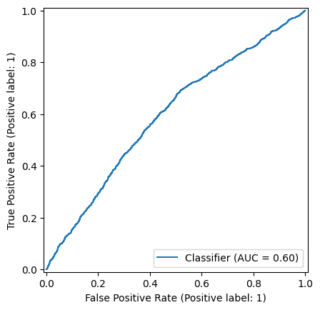
Để đánh giá model chúng ta cần sử dụng các metric như ROC, Accuracy, F1, precision hoặc recal.
Do dữ liệu không có hiện tượng mất cân bằng giữa 2 lớp nên ta sẽ sử dụng
ROClàm metric đánh giá model. Trong trường hợp mẫu mất cân bằng thì các chỉ sốF1,precisionhoặcrecalnên được sử dụng thay thế vì trong tình huống nàyROC,Accuracythường mặc định là rất cao.
Chúng ta sử dụng class BinaryClassificationEvaluator trong pyspark.ml.evaluation module để tính toán các metrics đánh giá model.
# Import the evaluation submodule
import pyspark.ml.evaluation as evals

# Create a BinaryClassificationEvaluator
evaluator = evals.BinaryClassificationEvaluator(metricName="areaUnderROC")
4.3.4.3. Tuning model thông qua param gridSearch#
Tuning model được hiểu là tìm kiếm trong 1 không gian các tham số của model để thu được model mà giá trị của metric khai báo ở bước 3.2.2 thu được là nhỏ nhất trên tập test
# Import the tuning submodule
import pyspark.ml.tuning as tune
import numpy as np

# Create the parameter grid - khởi tạo grid
grid = tune.ParamGridBuilder()

# Add the hyperparameter, we can add more than one hyperparameter
grid = grid.addGrid(lr.regParam, np.arange(0, 0.1, 0.01))
# có thể add thêm nhiều tham số khác : grid = grid.addGrid(<tham số>, <list value của tham số>)

# Build the grid - khởi tạo gridSearch
grid = grid.build()
# khởi tạo một cross validator từ class CrossValidator của pyspark.ml.tuning
# Create the CrossValidator
cv = tune.CrossValidator(
    estimator=lr, estimatorParamMaps=grid, evaluator=evaluator
)

# Fit cross validation on models
models = cv.fit(train)
# model tốt nhất
best_lr = models.bestModel

# Lưu ý để dự báo từ các model của pyspark, chúng ta không sử dụng hàm predict() như thông thường mà sử dụng hàm transform().
test_results = best_lr.transform(test)

# Kiểm tra mức độ chính xác của model trên tập test bằng hàm evaluate()
print(evaluator.evaluate(test_results))
0.5958682645678443
test.show(5)
+-------------+------------+-----+----+-----------+-------------------+-------+--------+-----+-----------------+----------------+-------------+-------------+--------------------+
|ARRIVAL_DELAY|ARRIVAL_TIME|MONTH|YEAR|DAY_OF_WEEK|DESTINATION_AIRPORT|AIRLINE|IS_DELAY|label|DESTINATION_INDEX|DESTINATION_FACT|AIRLINE_INDEX| AIRLINE_FACT|            features|
+-------------+------------+-----+----+-----------+-------------------+-------+--------+-----+-----------------+----------------+-------------+-------------+--------------------+
|           -1|         620|    3|2015|          2|                ATL|     DL|   false|    0|              1.0|  (24,[1],[1.0])|          0.0|(1,[0],[1.0])|(29,[0,1,2,3,5,28...|
|           -1|         825|    1|2015|          7|                MIA|     AA|   false|    0|             13.0| (24,[13],[1.0])|          1.0|    (1,[],[])|(29,[0,1,2,3,17],...|
|           -1|        1024|    1|2015|          7|                SLC|     DL|   false|    0|              2.0|  (24,[2],[1.0])|          0.0|(1,[0],[1.0])|(29,[0,1,2,3,6,28...|
|           -1|        1122|    3|2015|          1|                HNL|     DL|   false|    0|             10.0| (24,[10],[1.0])|          0.0|(1,[0],[1.0])|(29,[0,1,2,3,14,2...|
|           -1|        1156|    3|2015|          7|                MSP|     DL|   false|    0|              3.0|  (24,[3],[1.0])|          0.0|(1,[0],[1.0])|(29,[0,1,2,3,7,28...|
+-------------+------------+-----+----+-----------+-------------------+-------+--------+-----+-----------------+----------------+-------------+-------------+--------------------+
only showing top 5 rows
df = test_results.toPandas()
df["label"].value_counts()
label
0    2428
1    1667
Name: count, dtype: int64
from sklearn.metrics import roc_curve, auc, roc_auc_score, RocCurveDisplay

RocCurveDisplay.from_predictions(
    df["label"], 1 - df["probability"].map(lambda x: x[0])
)
<sklearn.metrics._plot.roc_curve.RocCurveDisplay at 0x28e5ab07f10>