2.3.1. Data-level approaches

Methods will change the data distribution by remove or adding more obs in raw dataset to balancing the class

2.3.1.1. Undersampling

Process of reducing the number of sample from the majority Class

• Balancing ratio: $\(R(x) = \frac{X_{minority}}{X_{majority}}\)$

Type of undersampling

• Fixed (reduce majority class to the same number of obs than minority): \(R(x) = 1\)

• Cleaning (clean the majority class bases on same criteria)

STT	Methods	Fixed vs Cleaning	Under-sampling criteria	Method of data Exclusion	Final Dataset Size
1	Random	Fixed	Random	Random	2 x minority class
2	NearMiss	Fixed	Keep boundary obs		2 x minority class
3	Instance Hardness	Fixed	Remove noise obs	Remove low probability class obs	2 x minority class
4	Condensed Nearest Neighbourhood (CNN)	Cleaning	Keep boundary obs	Samples outside the boundary between the classes	Varies
5	Tomek Links	Cleaning	Remove noise obs	Samples are Tomek Links	Varies
6	One Sided	Cleaning	Keep boundary + remove noise	CNN + Tomek Links	Varies
7	Edited Nearest Neighbourhood (ENN)	Cleaning	Remove noise obs	Observation’s class is different from that of its nearest neighbours	Varies
8	Repeated ENN	Cleaning	Remove noise obs	Repeats ENN multiple times	Varies
9	Neighbourhood Clearning Rule (NCR)	Cleaning	Remove noise obs		Varies
10	All KNN	Cleaning	Remove noise obs	Repeats ENN, plus 1 neighbour in each KNN iteration	Varies

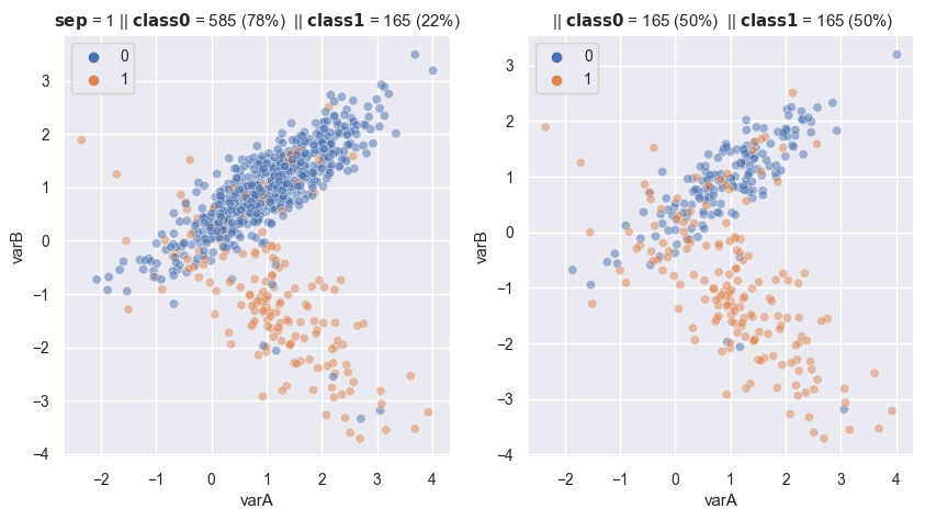
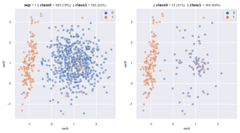
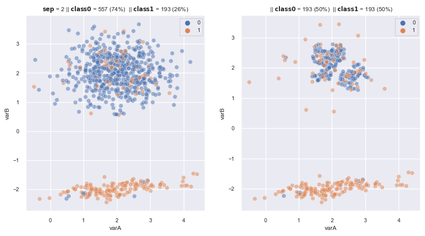
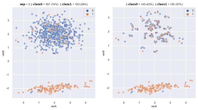
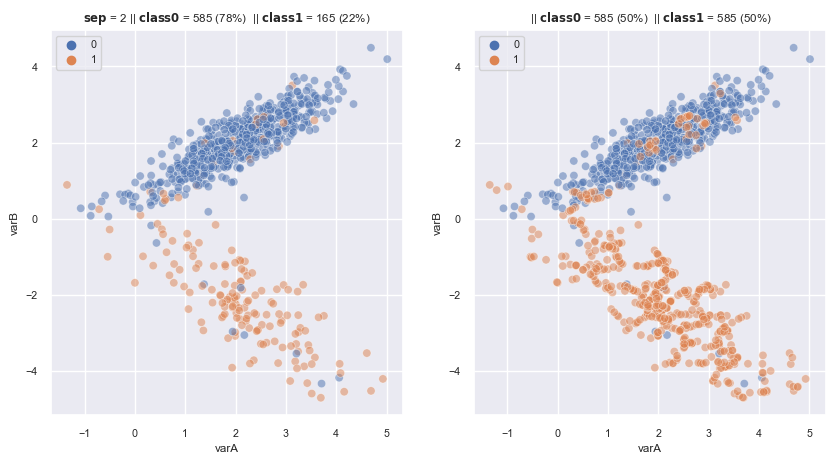
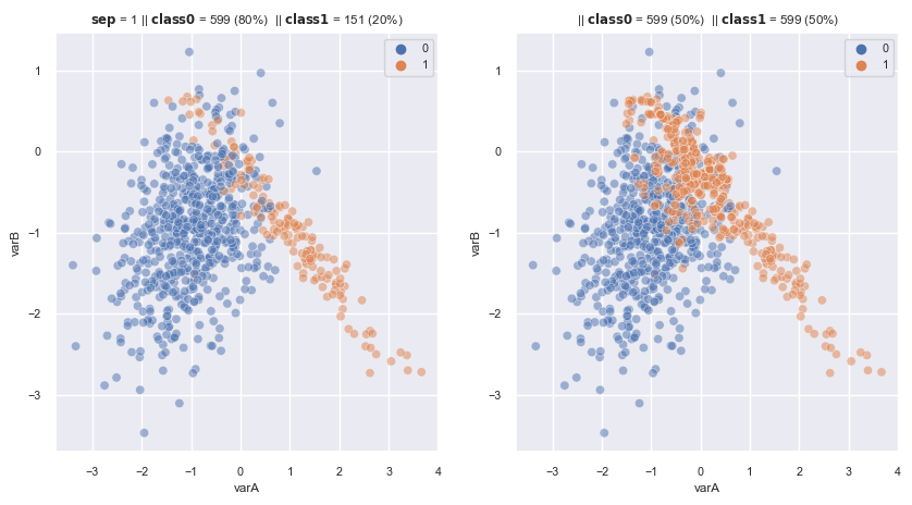
2.3.1.1.1. Random undersampling

Remove random majority class obs until \(R(x)\) =1

Methods	Fixed vs Cleaning	Under-sampling criteria	Method of data Exclusion	Final Dataset Size
Random	Fixed	Random	Random	2 x minority class

• Criteria for data exclusion: Random

• Final Dataset size: 2 x minority class

• Assumption: None

• Model Performance:

  • Make good balance of each class, so model do not just learning focus only majority class.

  • Remove importance Information and obs, so model is harder to learn patterns to differentiate the classes

• Application:

  • Large and not highly imbalance dataset

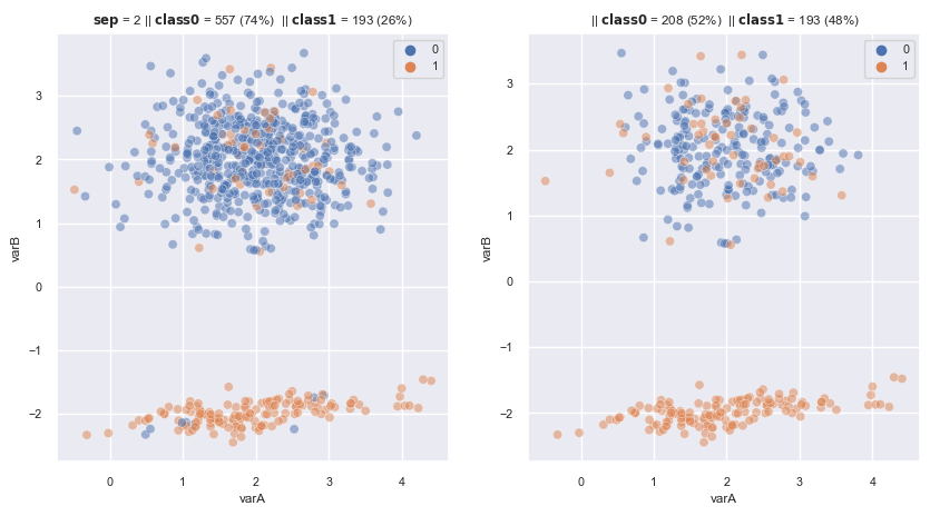
from imblearn.under_sampling import RandomUnderSampler

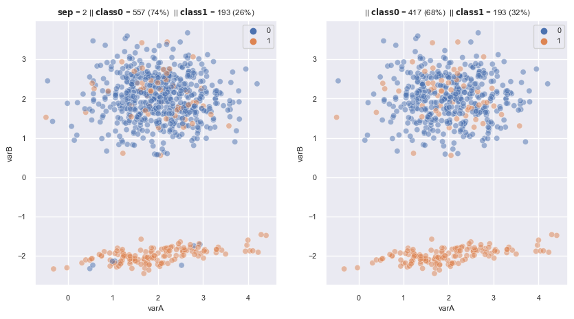
With balanced ratio

# R(x) = 1
fig, axes = plt.subplots(1, 2, sharex=True, figsize=(10,5))
X, y = make_data(1, ax = axes[0])

rus = RandomUnderSampler(
                    sampling_strategy='auto', 
                    replacement=False , # replacement resample or not
                        )
X_re, y_re = rus.fit_resample(X,y)
scat_plot(X_re, y_re, ax = axes[1])

<Figure size 500x500 with 0 Axes>

<Figure size 500x500 with 0 Axes>

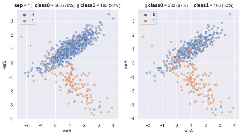
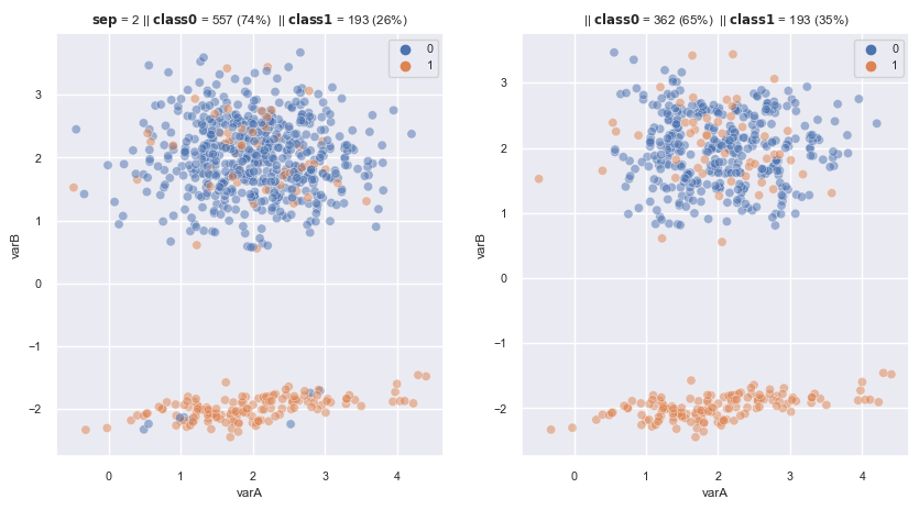
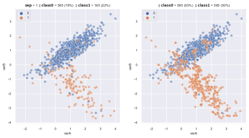
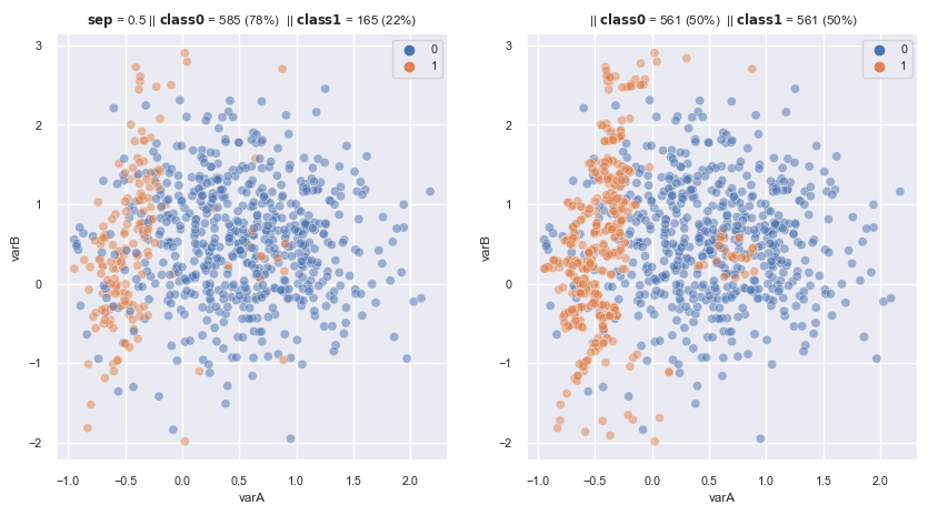
With specific balance ratio

# Changing the balancing ratio

fig, axes = plt.subplots(1, 2, sharex=True, figsize=(10,5))
X, y = make_data(1, ax = axes[0])

rus = RandomUnderSampler(
                    sampling_strategy= 0.5, # remember balancing ratio = x min / x maj
                    replacement=False , # replacement resample or not
                        )
X_re, y_re = rus.fit_resample(X,y)
scat_plot(X_re, y_re, ax = axes[1])

<Figure size 500x500 with 0 Axes>

<Figure size 500x500 with 0 Axes>

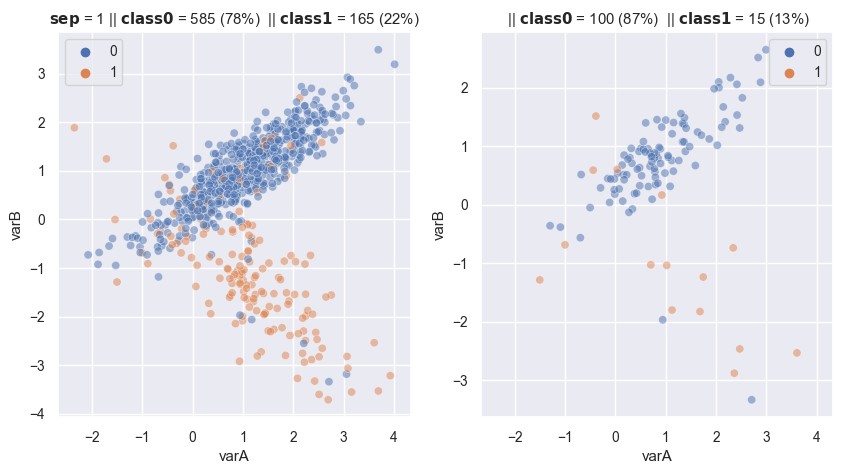
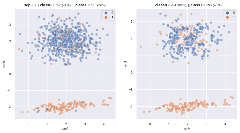
Specify number of observations in each class

# specify number of observations in each class

fig, axes = plt.subplots(1, 2, sharex=True, figsize=(10,5))
X, y = make_data(1, ax = axes[0])

rus = RandomUnderSampler(
                    sampling_strategy= {0:100, 1:15},
                    replacement=False , # replacement resample or not
                        )
X_re, y_re = rus.fit_resample(X,y)
scat_plot(X_re, y_re, ax = axes[1])

<Figure size 500x500 with 0 Axes>

<Figure size 500x500 with 0 Axes>

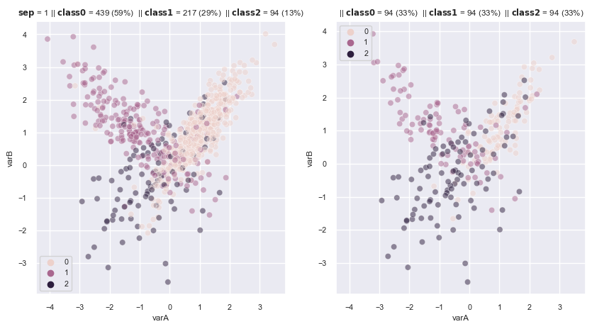
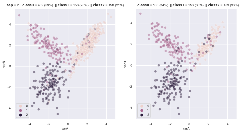
In multi class

# multi class
# R(x) = 1
sns.set(font_scale=0.7)
fig, axes = plt.subplots(1, 2, sharex=True, figsize=(10,5))
X, y = make_data(1, weights=[0.6, 0.3, 0.1],  ax = axes[0])

rus = RandomUnderSampler(
                    sampling_strategy='auto', 
                    replacement=False , # replacement resample or not
                        )
X_re, y_re = rus.fit_resample(X,y)
scat_plot(X_re, y_re, ax = axes[1])

<Figure size 500x500 with 0 Axes>

<Figure size 500x500 with 0 Axes>

2.3.1.1.2. Condensed Nearest Neighbourhood (CNN)

Select obs are near the boundary between the classes by KNN:

• If the classes are similar, the final selection sample would contain a pair amount for each class

• If the classes are seem different, the final selection sample would contain mostly 1 class (the minority class)

Methods	Fixed vs Cleaning	Under-sampling criteria	Method of data Exclusion	Final Dataset Size
Condensed Nearest Neighbourhood (CNN)	Cleaning	Keep boundary obs	Samples outside the boundary between the classes	Varies

---

The algorithms works as follows:

1. Put all minority class observations in a group, typically group O

2. Add 1 observation (at random) from the majority class to group O

3. Train a KNN with group O

4. Take 1 observation of the majority class that is not in group O yet

5. Predict its class with the KNN from point 3

   • If the prediction was correct, then ignore this observation and go to 4 and repeat

   • If the prediction was incorrect, add this observation to group O, go to 3 and repeat

6. Continue until all samples of the majority class were either assigned to O or left out

7. Final version of Group O is our undersampled dataset

---

• Criteria for data exclusion: Keep boundary obs

• Assumption: None

• Model Performance:

  • Make distort the data distribution and tends to add noise (uncertain class) to undersampled data (select points that are near other classes)

  • But because learning from this hardest datapoint so model successfull to learn patterns class, so better to classify.

  • Computationally expensive, because it trains 1 KNN every time an observation is added to the minority class group.

  • Randomness because select random first observation from majority class and put it to O

  • Support OnevsRest approach for multiclass (splitting to multiple binary-class)

• Application:

from imblearn.under_sampling import CondensedNearestNeighbour

fig, axes = plt.subplots(1, 2, sharex=True, figsize=(10,5))
X, y = make_data(1, random_state=3, flip_y=0.05 , ax = axes[0])

cnn = CondensedNearestNeighbour(
    sampling_strategy='auto',  # undersamples only the majority class
    random_state=0,  # for reproducibility
    n_neighbors=1,# default
    n_jobs=4)  

X_re, y_re = cnn.fit_resample(X,y)
scat_plot(X_re, y_re, ax = axes[1])

<Figure size 500x500 with 0 Axes>

<Figure size 500x500 with 0 Axes>

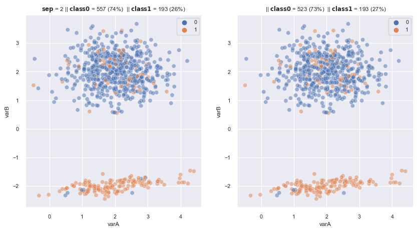
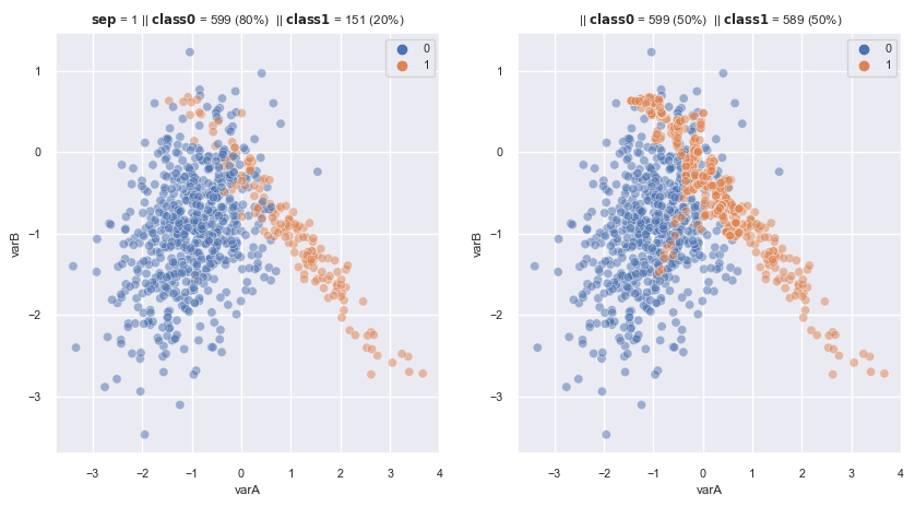
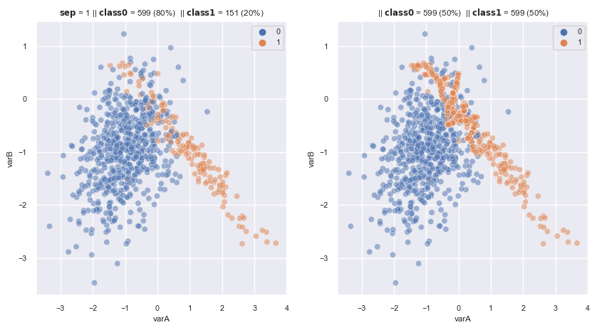
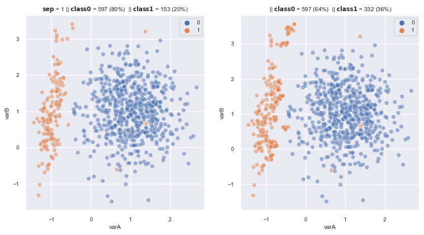
2.3.1.1.3. Tomek Links

Remove the obs that are tomek links, 2 obs are nearest neighbours and from different class. This procedures will remove 1 of 2 tomek links, which is in majority class or both of them. –> Remove những obs thuộc majority class và near với minority class

Methods	Fixed vs Cleaning	Under-sampling criteria	Method of data Exclusion	Final Dataset Size
Tomek Links	Cleaning	Remove noise obs	Samples are Tomek Links	Varies

---

• Assumption: Boundary is noise

• Model Performance:

  • Make distort the data distribution

  • May be remove noise and improves performance

  • Poor to classify the hard-case obs

  • Support OnevsRest approach for multiclass (splitting to multiple binary-class)

• Application:

from imblearn.under_sampling import TomekLinks

fig, axes = plt.subplots(1, 2, sharex=True, figsize=(10,5))
X, y = make_data(2, random_state=3, flip_y=0.15 , ax = axes[0])

tl1 = TomekLinks(sampling_strategy='auto')  # undersamples only the majority class
tl2 = TomekLinks(sampling_strategy='all')  # remove both majority and minority obs in tomek links
 

X_re, y_re = tl1.fit_resample(X,y)
scat_plot(X_re, y_re, ax = axes[1])

<Figure size 500x500 with 0 Axes>

<Figure size 500x500 with 0 Axes>

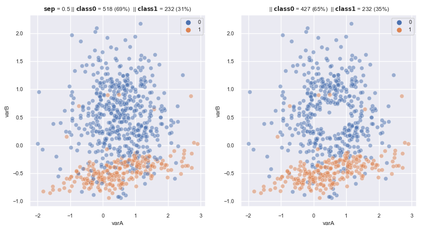
2.3.1.1.4. One Sided Selection

Combine 2 methods CNN and Tomek links by select first samples at the boundary of the classes using CNN then removes the tomek links. –> Focus only on harder cases by selecting those at the boundary, while removing noise (maybe) with tomek links

Methods	Fixed vs Cleaning	Under-sampling criteria	Method of data Exclusion	Final Dataset Size
One Sided Selection	Cleaning	Keep boundary + remove noise	CNN + Tomek Links	Varies

---

• Assumption:

• Model Performance:

  • Make distort the data distribution

  • May be remove noise and focus to clearn classify hardest case data, then improves performance

  • Support OnevsRest approach for multiclass (splitting to multiple binary-class)

• Application:

from imblearn.under_sampling import OneSidedSelection

fig, axes = plt.subplots(1, 2, sharex=True, figsize=(10,5))
X, y = make_data(0.5, random_state=3, flip_y=0.03 , ax = axes[0], weights=[0.7, 0.3])

oss = OneSidedSelection(
    sampling_strategy='auto',  # undersamples only the majority class
    random_state=0,  # for reproducibility
    n_neighbors=1,# default
    n_jobs=4)
 

X_re, y_re = oss.fit_resample(X,y)
scat_plot(X_re, y_re, ax = axes[1])

<Figure size 500x500 with 0 Axes>

<Figure size 500x500 with 0 Axes>

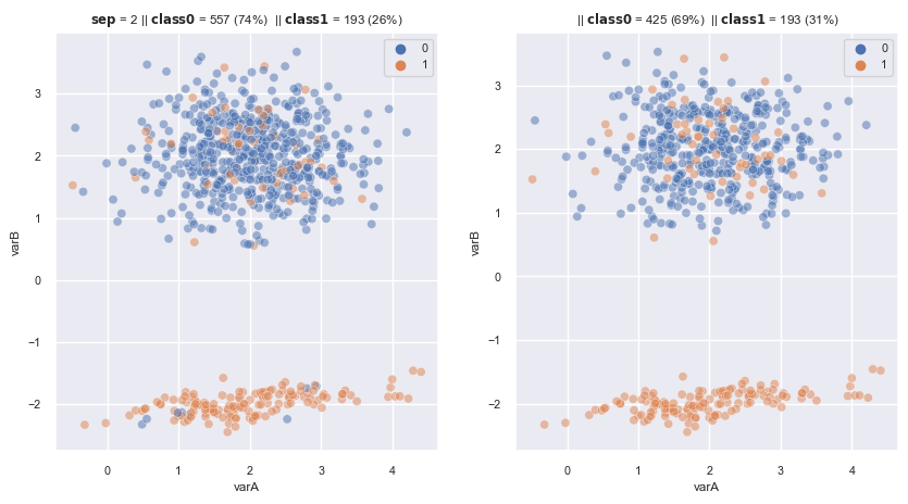
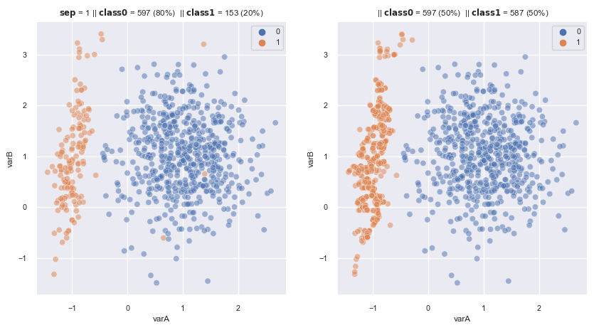
2.3.1.1.5. Edited Nearest Neighbours

Removes observations which class are different from that of their neighbours. These are generally the observations difficult to classify and / or that introduce noise. ENN is the opposite of Condensed NN

–> In practice, samples of the majority class that are too similar to an observation of the minority class will be removed

Methods	Fixed vs Cleaning	Under-sampling criteria	Method of data Exclusion	Final Dataset Size
Edited Nearest Neighbourhood (ENN)	Cleaning	Remove noise obs	Observation’s class is different from that of its nearest neighbours	Varies

---

The algorithms works as follows:

1. For each observation in dataset, find the k nearest neighbour to each observation (typically k=3)

• If the majority class of k (mode strategy) or all class of k (all strategy) is the same class of that datapoint, then keep datapoint, else set mark ‘remove datapoint’

2. Do step1 for all observations dataset, then remove all datapoint which mark ‘remove datapoint’

---

• Assumption:

• Model Performance:

  • Make distort the data distribution

  • Remove hard-case obs (data point is uncasual)

• Application:

from imblearn.under_sampling import EditedNearestNeighbours

fig, axes = plt.subplots(1, 2, sharex=True, figsize=(10,5))
X, y = make_data(2, random_state=3, flip_y=0.15 , ax = axes[0])

enn = EditedNearestNeighbours(
    sampling_strategy='auto',  # undersamples only the majority class
    n_neighbors=3, # the number of neighbours to examine
    kind_sel='all',  # all neighbours need to have the same label as the observation examined
    n_jobs=4)

X_re, y_re = enn.fit_resample(X,y)
scat_plot(X_re, y_re, ax = axes[1])

<Figure size 500x500 with 0 Axes>

<Figure size 500x500 with 0 Axes>

2.3.1.1.6. Repeated Edited Nearest Neighbours

Extends Edited Nearest neighbours in that it repeats the procedure over an over with the same K, until no further observation is removed from the dataset, or alternatively until a maximum number of iterations is reached.

Methods	Fixed vs Cleaning	Under-sampling criteria	Method of data Exclusion	Final Dataset Size
Repeated ENN	Cleaning	Remove noise obs	Repeats ENN multiple times	Varies

---

• Assumption:

• Model Performance:

  • Make distort the data distribution

  • Remove hard-case obs (data point is uncasual)

  • Remove more obs than ENN

• Application:

from imblearn.under_sampling import RepeatedEditedNearestNeighbours


renn = RepeatedEditedNearestNeighbours(
    sampling_strategy='auto',# removes only the majority class
    n_neighbors=3, # the number of neighbours to examine
    kind_sel='all', # all neighbouring observations should show the same class
    n_jobs=4, # 4 processors in my laptop
    max_iter=100) # maximum number of iterations

fig, axes = plt.subplots(1, 2, sharex=True, figsize=(10,5))
X, y = make_data(2, random_state=3, flip_y=0.15 , ax = axes[0])

X_re, y_re = renn.fit_resample(X,y)
scat_plot(X_re, y_re, ax = axes[1])

<Figure size 500x500 with 0 Axes>

<Figure size 500x500 with 0 Axes>

2.3.1.1.7. All KNN

Similar RENN but at each round, K increases 1 neighbours:

• Start K = 1

• End K = max K (defined by user) or if the majority class becomes the minority

Methods	Fixed vs Cleaning	Under-sampling criteria	Method of data Exclusion	Final Dataset Size
All KNN	Cleaning	Remove noise obs	Repeats ENN, plus 1 neighbour in each KNN iteration	Varies

---

• Assumption:

• Model Performance:

  • Make distort the data distribution

  • Remove hard-case obs (data point is uncasual)

  • Remove more obs than ENN

  • The criteria of obs to be retain harder and harder after each round, therefore removing more observations that are closer to the boundary to the minority class.

• Application:

  • ENN, RENN and AllKNN tend to produce similar results, so we may as well just choose one of the 3

from imblearn.under_sampling import  AllKNN

allknn = AllKNN(
    sampling_strategy='auto',  # undersamples only the majority class
    n_neighbors=5, # the maximum size of the neighbourhood to examine
    kind_sel='all',  # all neighbours need to have the same label as the observation examined
    n_jobs=4)  # I have 4 cores in my laptop

fig, axes = plt.subplots(1, 2, sharex=True, figsize=(10,5))
X, y = make_data(2, random_state=3, flip_y=0.15 , ax = axes[0])

X_re, y_re = allknn.fit_resample(X,y)
scat_plot(X_re, y_re, ax = axes[1])

<Figure size 500x500 with 0 Axes>

<Figure size 500x500 with 0 Axes>

2.3.1.1.8. Neighbourhood Cleaning Rule

Combine ENN + KNN rule for each 3 neighbours of each obs minority class

Methods	Fixed vs Cleaning	Under-sampling criteria	Method of data Exclusion	Final Dataset Size
Neighbourhood Clearning Rule (NCR)	Cleaning	Remove noise obs	ENN mode strategy + rule for 3 neighbours of minority obs	Varies

---

The Neighbourhood Cleaning Rule works as follows:

1. For each majority class obs, use ENN with mode strategy to remove or not.

2. For minority class, check 3 its neighbours and remove a neighbours if it satisfies all three conditions at the same time:

• This datapoint belong to majoity class:

• The other neighbours are not the same class with this neighbour

• The majority class has at least half as many observations as those in the minority (this can be regulated)

---

• Assumption:

• Model Performance:

  • Make distort the data distribution

  • Remove hard-case majority obs (data point is uncasual)

  • Remove more obs than ENN

from imblearn.under_sampling import NeighbourhoodCleaningRule

ncr = NeighbourhoodCleaningRule(
    sampling_strategy='auto',# undersamples from all classes except minority
    n_neighbors=3, # explores 3 neighbours per observation
    kind_sel='all', # all neighbouring need to disagree, only applies to cleaning step
                    # set 'mode' then most neighbours need to disagree to be removed.
    n_jobs=4, # 4 processors in my laptop
    threshold_cleaning=0.5, # the threshold to evaluate a class for cleaning (used only for clearning step)
) 

fig, axes = plt.subplots(1, 2, sharex=True, figsize=(10,5))
X, y = make_data(2, random_state=3, flip_y=0.15 , ax = axes[0])

X_re, y_re = ncr.fit_resample(X,y)
scat_plot(X_re, y_re, ax = axes[1])

<Figure size 500x500 with 0 Axes>

<Figure size 500x500 with 0 Axes>

2.3.1.1.9. Near Miss

• Select (retains) obs that are somewhat similar to the minority class, using 1 of three alternative procedures:

  1. Select majority ob that has the average distance to k-closest minority obs is smallest

  2. Select majority ob that has the average distance to k-farthest minority obs is smallest

  3. From these majority obs in which is the 1 of K closest datapoint of at least 1 minority class, select majority ob that has the average distance to k-farthest minority obs is smallest

• Design to work with text, where each work is a complex representation of works and tags

Methods	Fixed vs Cleaning	Under-sampling criteria	Method of data Exclusion	Final Dataset Size
NearMiss	Fixed	Keep boundary obs		2 x minority class

from imblearn.under_sampling import NearMiss


nm1 = NearMiss(
    sampling_strategy='auto',  # undersamples only the majority class
    version=1,
    n_neighbors=3,
    n_jobs=4)  # I have 4 cores in my laptop

fig, axes = plt.subplots(1, 2, sharex=True, figsize=(10,5))
X, y = make_data(2, random_state=3, flip_y=0.15 , ax = axes[0])

X_re, y_re = nm1.fit_resample(X,y)
scat_plot(X_re, y_re, ax = axes[1])

<Figure size 500x500 with 0 Axes>

<Figure size 500x500 with 0 Axes>

nm2 = NearMiss(
    sampling_strategy='auto',  # undersamples only the majority class
    version=2,
    n_neighbors=3,
    n_jobs=4)  # I have 4 cores in my laptop

fig, axes = plt.subplots(1, 2, sharex=True, figsize=(10,5))
X, y = make_data(2, random_state=3, flip_y=0.15 , ax = axes[0])

X_re, y_re = nm2.fit_resample(X,y)
scat_plot(X_re, y_re, ax = axes[1])

<Figure size 500x500 with 0 Axes>

<Figure size 500x500 with 0 Axes>

nm3 = NearMiss(
    sampling_strategy='auto',  # undersamples only the majority class
    version=3,
    n_neighbors=3,
    n_jobs=4)  # I have 4 cores in my laptop

fig, axes = plt.subplots(1, 2, sharex=True, figsize=(10,5))
X, y = make_data(2, random_state=3, flip_y=0.15 , ax = axes[0])

X_re, y_re = nm3.fit_resample(X,y)
scat_plot(X_re, y_re, ax = axes[1])

<Figure size 500x500 with 0 Axes>

<Figure size 500x500 with 0 Axes>

2.3.1.1.10. Instance Hardness

• Instance Hardness Threshold: the probability of an observation being miss-classified. So in other words, the instance hardness is 1 minus the probability of the class.

  • For class 1: instance hardness = 1 - P(X = 1)

• Instance Hardness Filtering: Removing the observations with high instance hardness (above threshold) or in other word that is low class probability. The probability are given by any classifier method and the threshold is calculated by: $\(threshold = 1 - \frac{\text{number of minority obs}}{\text{number of majority obs}}\)$

Methods	Fixed vs Cleaning	Under-sampling criteria	Method of data Exclusion	Final Dataset Size
Instance Hardness	Fixed	Remove noise obs	Remove low probability class obs	2 x minority class

from imblearn.under_sampling import InstanceHardnessThreshold
from sklearn.ensemble import RandomForestClassifier

# binary
rf = RandomForestClassifier(n_estimators=5, random_state=1, max_depth=2)

iht = InstanceHardnessThreshold(
    estimator=rf,
    sampling_strategy='auto',  # undersamples only the majority class
    random_state=1,
    n_jobs=4, # have 4 processors in my laptop
    cv=3,  # cross validation fold
)

fig, axes = plt.subplots(1, 2, sharex=True, figsize=(10,5))
X, y = make_data(2, random_state=3, flip_y=0.15 , ax = axes[0])

X_re, y_re = iht.fit_resample(X,y)
scat_plot(X_re, y_re, ax = axes[1])

<Figure size 500x500 with 0 Axes>

<Figure size 500x500 with 0 Axes>

# multiclass
sns.set(font_scale=0.7)
from sklearn.multiclass import OneVsRestClassifier

rf = OneVsRestClassifier(
    RandomForestClassifier(n_estimators=10, random_state=1, max_depth=2),
    n_jobs=4,
)

iht = InstanceHardnessThreshold(
    estimator=rf,
    sampling_strategy='auto',  # undersamples all majority classes
    random_state=1,
    n_jobs=4, # have 4 processors in my laptop
    cv=3,  # cross validation fold
)

fig, axes = plt.subplots(1, 2, sharex=True, figsize=(10,5))
X, y = make_data(2, weights=[0.6, 0.2, 0.2], flip_y=0.1 , ax = axes[0])

X_re, y_re = iht.fit_resample(X,y)
scat_plot(X_re, y_re, ax = axes[1])

<Figure size 500x500 with 0 Axes>

<Figure size 500x500 with 0 Axes>

2.3.1.2. Oversampling

Process of increasing the number of obs from the minority Class

• Balancing ratio: $\(R(x) = \frac{X_{minority}}{X_{majority}}\)$

Type of oversampling

• Extraction (extracts random obs fromo minority class): Random

• Generation (Creates new obs that slightly different from existing ones ): SMOTE, ADASYN,…:

  • All obs as templates: SMOTE, SMOTE-NC

  • Focus to generate from obs closer to the boundary with the majority class: SMOTE variants, ADASYN,…

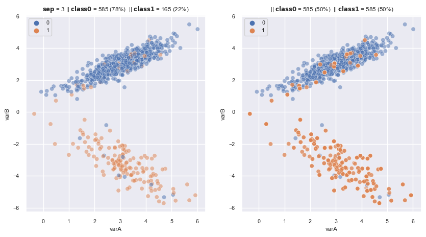
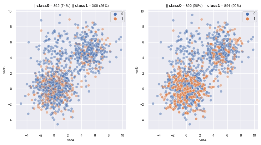
2.3.1.2.1. Random oversampling

Extracts obs at random from the minority with replacement class until a certain \(R(x)\) is reached

• Duplicates obs from the minority class –> Increase likelihood overfitting

• In order not to DUPLICATE the data, after extracting the samples at random, we multiply the value of the sample by a number that contemplates the dispersion of the data, to obtain artificial examples. (ROS with Smoothing)

from imblearn.over_sampling import RandomOverSampler

fig, axes = plt.subplots(1, 2, sharex=True, figsize=(10,5))
X, y = make_data(3, ax = axes[0])

ros = RandomOverSampler(
    sampling_strategy='auto', # samples only the minority class
    random_state=0,  # for reproducibility
)  

X_re, y_re = ros.fit_resample(X,y)
scat_plot(X_re, y_re, ax = axes[1])

<Figure size 500x500 with 0 Axes>

<Figure size 500x500 with 0 Axes>

# Random overresampling with smoothing
ros_sm = RandomOverSampler(
    sampling_strategy='auto', # samples only the minority class
    random_state=0,  # for reproducibility
    shrinkage = 0.5,
)  

fig, axes = plt.subplots(1, 2, sharex=True, figsize=(10,5))
X, y = make_data(3, ax = axes[0])

X_re, y_re = ros_sm.fit_resample(X,y)
scat_plot(X_re, y_re, ax = axes[1])

<Figure size 500x500 with 0 Axes>

<Figure size 500x500 with 0 Axes>

2.3.1.2.2. SMOTE

Synthetic minority Over-sampling Technique

For each minority observation X, find k nearest minority neighbours (typically 5), choose a random neighbour from 5 and interpolate a new obs among X and this nearest neighbours by multiplies that distance to each neighbour with random number, then add a new obs to dataset

• New obs from minority class will not be identical to original ones (prevent duplication)

• SMOTE suitable for numeric continuous, use SMOTE-NC for categorical

from imblearn.over_sampling import SMOTE

sm = SMOTE(
    sampling_strategy='auto',  # samples only the minority class
    random_state=0,  # for reproducibility
    k_neighbors=5
)

fig, axes = plt.subplots(1, 2, sharex=True, figsize=(10,5))
X, y = make_data(2, ax = axes[0])

X_re, y_re = sm.fit_resample(X,y)
scat_plot(X_re, y_re, ax = axes[1])

<Figure size 500x500 with 0 Axes>

<Figure size 500x500 with 0 Axes>

2.3.1.2.3. SMOTE-NC

Extends the funcitonality of SMOTE to categorical variables:

• The distance function is L2 Euclidean distances:

  • for numberic variables, calculate in casual

  • for categorical:

    • if the same value, replace by 0

    • if differ value, replace by the median value of list standard deviation of all numeric variables

• How to mark category label in new minority obs?

  • mark by the majority label of k nearest neighbor of new obs.

from imblearn.over_sampling import SMOTENC
import random

foo = ['a', 'b', 'c', 'd', 'e']
smnc = SMOTENC(
    sampling_strategy='auto', # samples only the minority class
    random_state=0,  # for reproducibility
    k_neighbors=5,
    n_jobs=4,
    categorical_features=[2,3] # indeces of the columns of categorical variables
)  

fig, axes = plt.subplots(1, 2, sharex=True, figsize=(10,5))
X, y = make_data(1, ax = axes[0])
X['cat1'] = [random.choice(foo) for i in range(len(X))]
X['cat2'] = [random.choice(foo) for i in range(len(X))]
X_re, y_re = smnc.fit_resample(X,y)
scat_plot(X_re, y_re, ax = axes[1])

<Figure size 500x500 with 0 Axes>

<Figure size 500x500 with 0 Axes>

2.3.1.2.4. ADASYN

• Like SMOTE, but use more hard-case to classify observation to generate new data and use KNN for all observation dataset (instead KNN for only minority obs like SMOTE)

• Because the weight is high if the minority obs has more majority neighbours in K nearest neighbours, so this method would create more new obs at boundary between minority class and majority class –> Model learn more pattern to classify

• ADASYN make distort the class shape

---

Procedure

1. Determine the Initial balance ratio \(R(x) = \frac{X_{minority}}{X_{majority}}\) and the amount of gerneration \(G = factor * (X_{maj} - X_{min}) \)

2. Train KNN for all obs dataset, find k nearest neighbour of each minority obs, and calculate the weight of majority class neighbours \(r = \frac{\text{number of majority neighbour}}{K}\)

3. Norm these weight \(r\) of all minority obs : \(r_{norm} = \frac{r}{sum(rs)}\)

4. Calculate the number of generation obs for each minority obs: \(g_i = r_i * G\)

5. For each minority obs i, create \(g_i\) new obs like SMOTE, but the neighbour would be either from majority class or minority class (unlike SMOTE: neighbours are only minority)

from imblearn.over_sampling import ADASYN

ada = ADASYN(
    sampling_strategy='auto',  # samples only the minority class
    random_state=0,  # for reproducibility
    n_neighbors=5,
    n_jobs=4
)

fig, axes = plt.subplots(1, 2, sharex=True, figsize=(10,5))
X, y = make_data(1, ax = axes[0], flip_y=0.01, random_state = 5)

X_re, y_re = ada.fit_resample(X,y)
scat_plot(X_re, y_re, ax = axes[1])

<Figure size 500x500 with 0 Axes>

<Figure size 500x500 with 0 Axes>

2.3.1.2.5. Borderline SMOTE

• Creates new obs by interpolation between obs of the minority class and their closest neighbours.

• It does not use all observations from the minority class as templates, unllike SMOTE.

Following step:

1. It selects those observations (from the minority) for which, most of their neighbours belong to a different class (DANGER group)

   • Note that: the minority which has all of k nearest neighbours belong to majority class, may be noise datapoint. Or the minority which has most of k nearest neighbours belong to minority class, is too safety and easy to classify –> not select this kind of minority obs

2. Generate new obs:

• Variant 1: creates new examples, as SMOTE, between samples in the Danger group and their closest neighbours from the minority

• Variant 2: creates new examples, similar SMOTE, but between samples in the Danger group and their closest neighbours from the majority

# variant 1
from imblearn.over_sampling import BorderlineSMOTE

sm_b1 = BorderlineSMOTE(
    sampling_strategy='auto',  # samples only the minority class
    random_state=0,  # for reproducibility
    k_neighbors=5, # the neighbours to crete the new examples (step2)
    m_neighbors=10, # the neiighbours to find the DANGER group (step1)
    kind='borderline-1', # variant 1
    n_jobs=4
)

fig, axes = plt.subplots(1, 2, sharex=True, figsize=(10,5))
X, y = make_data(1, ax = axes[0], flip_y=0.01, random_state = 5)

X_re, y_re = sm_b1.fit_resample(X,y)
scat_plot(X_re, y_re, ax = axes[1])

<Figure size 500x500 with 0 Axes>

<Figure size 500x500 with 0 Axes>

# variant 2
sm_b2 = BorderlineSMOTE(
    sampling_strategy='auto',  # samples only the minority class
    random_state=0,  # for reproducibility
    k_neighbors=5, # the neighbours to crete the new examples (step2)
    m_neighbors=10, # the neiighbours to find the DANGER group (step1)
    kind='borderline-2', 
    n_jobs=4
)

fig, axes = plt.subplots(1, 2, sharex=True, figsize=(10,5))
X, y = make_data(1, ax = axes[0], flip_y=0.01, random_state = 5)

X_re, y_re = sm_b2.fit_resample(X,y)
scat_plot(X_re, y_re, ax = axes[1])

<Figure size 500x500 with 0 Axes>

<Figure size 500x500 with 0 Axes>

2.3.1.2.6. SVM SMOTE

Extension of SMOTE : generate new obs for minority obs, that close to the boundary given by SVM

• if most neighbours are belong to minority class, use extrapolation to expand the boundary

• if most neighbours are belong to majority class, use interpolation to narrow the boundary

from imblearn.over_sampling import SVMSMOTE
from sklearn import svm

sm = SVMSMOTE(
    sampling_strategy='auto',  # samples only the minority class
    random_state=0,  # for reproducibility
    k_neighbors=5, # neighbours to create the synthetic examples
    m_neighbors=10, # neighbours to determine if minority class is in "danger"
    n_jobs=4,
    svm_estimator = svm.SVC(kernel='linear')
)

fig, axes = plt.subplots(1, 2, sharex=True, figsize=(10,5))
X, y = make_data(1, random_state=3, flip_y=0.01 , ax = axes[0])

X_re, y_re = sm.fit_resample(X,y)
scat_plot(X_re, y_re, ax = axes[1])

<Figure size 500x500 with 0 Axes>

<Figure size 500x500 with 0 Axes>

2.3.1.2.7. Kmean SMOTE

• Oversampling for clusters which have enough minority obs, avoid create new minority in cluster in that almost non-exist that minority.

• Suitable for data have more than 1 cluster

Steps:

1. Find clusters by Kmeans with entire dataset (need to an idea of number of clusters there are in our data)

2. Select cluster with those which %minority > threshold

3. For each selected cluster:

   • Calculate L2mean = Mean Euclidean distance betwwen minority obs

   • Density = (number of minority obs) / L2mean

   • Sparsity = 1/density = mức độ rời rạc của các quan sát minority in cluster

   • Cluster sparsity weight = Sparsity / sum(Sparsity all clusters)

   • Number need to generate for this cluster: gi = Cluster sparsity weight * Total number need to generate

from sklearn.datasets import make_blobs
import numpy as np

def make_data2(ax = None):
    # Configuration options
    blobs_random_seed = 42
    centers = [(0, 0), (5, 5), (0,5)]
    cluster_std = 1.5
    num_features_for_samples = 2
    num_samples_total = 2100

    # Generate X
    X, y = make_blobs(
        n_samples=num_samples_total,
        centers=centers,
        n_features=num_features_for_samples,
        cluster_std=cluster_std)

    # transform arrays to pandas formats
    X = pd.DataFrame(X, columns=['varA', 'varB'])
    y = pd.Series(y)

    # different number of samples per blob
    X = pd.concat([
        X[y == 0],
        X[y == 1].sample(400, random_state=42),
        X[y == 2].sample(100, random_state=42)
    ], axis=0)

    y = y.loc[X.index]

    # reset indexes
    X.reset_index(drop=True, inplace=True)
    y.reset_index(drop=True, inplace=True)


    # create imbalanced target
    y = pd.concat([
        pd.Series(np.random.binomial(1, 0.3, 700)),
        pd.Series(np.random.binomial(1, 0.2, 400)),
        pd.Series(np.random.binomial(1, 0.1, 100)),
    ], axis=0).reset_index(drop=True)
    scat_plot(X, y, ax = ax)
    return X, y

from sklearn.cluster import KMeans
from imblearn.over_sampling import KMeansSMOTE

sm = KMeansSMOTE(
    sampling_strategy='auto',  # samples only the minority class
    random_state=0,  # for reproducibility
    k_neighbors=2,
    n_jobs=None,
    kmeans_estimator=KMeans(n_clusters=3, random_state=0),
    cluster_balance_threshold=0.1, # min of % minority in selected clusters
    density_exponent='auto'
)

fig, axes = plt.subplots(1, 2, sharex=True, figsize=(10,5))
X, y = make_data2(ax = axes[0])

X_re, y_re = sm.fit_resample(X,y)
scat_plot(X_re, y_re, ax = axes[1])

<Figure size 500x500 with 0 Axes>

<Figure size 500x500 with 0 Axes>

2.3.1.3. Combine Under and Oversampling

Combined used of SMOTE and ENN or Tomek Links to amplify the minority class and remove noisy observations that might be created.

from imblearn.under_sampling import EditedNearestNeighbours, TomekLinks
from imblearn.over_sampling import SMOTE
from imblearn.combine import SMOTEENN, SMOTETomek

# SMOTE + ENN

sm = SMOTE(
    sampling_strategy='auto',  # samples only the minority class
    random_state=0,  # for reproducibility
    k_neighbors=5,
    n_jobs=4
)

enn = EditedNearestNeighbours(
    sampling_strategy='auto',
    n_neighbors=3,
    kind_sel='all',
    n_jobs=4)

smenn = SMOTEENN(
    sampling_strategy='auto',  # samples only the minority class
    random_state=0,  # for reproducibility
    smote=sm,
    enn=enn,
)

fig, axes = plt.subplots(1, 2, sharex=True, figsize=(10,5))
X, y = make_data(1, random_state=3, flip_y=0.01 , ax = axes[0])

X_re, y_re = smenn.fit_resample(X,y)
scat_plot(X_re, y_re, ax = axes[1])

<Figure size 500x500 with 0 Axes>

<Figure size 500x500 with 0 Axes>

# SMOTE + Tomek link

sm = SMOTE(
    sampling_strategy='auto',  # samples only the minority class
    random_state=0,  # for reproducibility
    k_neighbors=5,
    n_jobs=4
)

tl = TomekLinks(
    sampling_strategy='all',
    n_jobs=4)

smtomek = SMOTETomek(
    sampling_strategy='auto',  # samples only the minority class
    random_state=0,  # for reproducibility
    smote=sm,
    tomek=tl,
)

fig, axes = plt.subplots(1, 2, sharex=True, figsize=(10,5))
X, y = make_data(0.5, random_state=3, flip_y=0.05 , ax = axes[0])

X_re, y_re = smtomek.fit_resample(X,y)
scat_plot(X_re, y_re, ax = axes[1])

<Figure size 500x500 with 0 Axes>

<Figure size 500x500 with 0 Axes>