2.2.5. Categorical Encoding#
How to transform/replace the category strings by a numerical representation, for the goal:
Produce variables that can be used to train model
To build predictive features form categories
1. Categorical Encoding Techniques
Traditional technniques:
One-hot encoding
Count/frequency encoding
Ordinal/Label encoding
Monotonic relationship (categorical variable and target are monotonic relationship - dong bien):
Ordered label encoding
Mean encoding
Weight of evidence
(Using monotonic can be improve the performance of linear models, or tree-base model, or if want to monotonic relationship between variable and target in model)
Rare labels:
One-hot encoding of frequent categories
Group rare label encoding
Alternative techniques:
Binary encoding
Feature hasing
Others
2. Techniques comparation
For
tree-base,one-hotencoding has a bad performance because it has a big feature spaceFor
logistic, thewoeencoding get the best performance.
Index |
Encoding Method |
Description |
Advantages |
Disadvantages |
Observations |
|---|---|---|---|---|---|
1 |
One Hot Encoding |
One hot encoding, consists in encoding each categorical variable with different boolean variables (also called dummy variables) which take values 0 or 1, indicating if a category is present in an observation. |
• Straightforward to implement |
• Expands the feature space |
Most machine learning algorithms, consider the entire data set while being fit. Therefore, encoding categorical variables into k - 1 binary variables, is better, as it avoids introducing redundant information. |
2 |
One Hot Encoding of Frequent/Top Categories |
Performing one hot encoding, only considering the most frequent categories |
• Straightforward to implement |
• Does not add any information that may make the variable more predictive |
The number of top variables is set arbitrarily. It could be 15, 10 or 5 as well. This number can be chosen arbitrarily or derived from data exploration. |
3 |
Integer Encoding |
Integer encoding consist in replacing the categories by digits from 1 to n (or 0 to n-1, depending the implementation), where n is the number of distinct categories of the variable. |
• Straightforward to implement |
• Does not capture any information about the categories labels |
• The numbers are assigned arbitrarily. |
4 |
Count or frequency encoding |
• Categories are replaced by the count or percentage of observations that show that category in the dataset. |
• Straightforward to implement |
• Not suitable for linear models |
|
5 |
Target guided encodings - Ordered ordinal encoding |
Categories are replaced by integers from 1 to k, where k is the number of distinct categories in the variable, but this numbering is informed by the mean of the target for each category. |
• Straightforward to implement |
• May lead to over-fitting |
• the encoding is guided by the target, and |
6 |
Target guided encodings - Mean encoding |
Mean encoding implies replacing the category by the average target value for that category. |
Same as Ordered Ordinal Encoding |
Same as Ordered Ordinal Encoding |
Same as Ordered Ordinal Encoding |
7 |
Target guided encodings - Probability Ratio Encoding |
For each category, we calculate the mean of target=1, that is the probability of the target being 1 ( P(1) ), and the probability of the target=0 ( P(0) ). And then, we calculate the ratio P(1)/P(0), and replace the categories by that ratio. |
Same as Ordered Ordinal Encoding |
Same as Ordered Ordinal Encoding |
Same as Ordered Ordinal Encoding |
8 |
Target guided encodings - Weight of evidence |
WoE = ln ( Distribution of Goods / Distribution of bads ) |
Same as Ordered Ordinal Encoding |
Same as Ordered Ordinal Encoding |
Same as Ordered Ordinal Encoding |
9 |
Rare Label Encoding |
Rare labels are those that appear only in a tiny proportion of the observations in a dataset |
• Grouping categories into rare for variables that show low cardinality may or may not improve model performance, however, we tend to re-group them into a new category to smooth model deployment. |
• Grouping infrequent labels or categories under a new category called ‘Rare’ or ‘Other’ is the common practice in machine learning for business |
# load data
import pandas as pd
from sklearn.model_selection import train_test_split

usecols = ["pclass", "sibsp", "parch", "sex", "embarked", "cabin", "survived"]
data = pd.read_csv("Datasets/titanic.csv", usecols=usecols)
data["cabin"] = data["cabin"].str[0]
data.fillna('Missing', inplace = True)

# let's separate into training and testing set
X_train, X_test, y_train, y_test = train_test_split( data.drop("survived", axis=1), data["survived"], test_size=0.3, random_state=0)
X_train.head()
| pclass | sex | sibsp | parch | cabin | embarked | |
|---|---|---|---|---|---|---|
| 501 | 2 | female | 0 | 1 | Missing | S |
| 588 | 2 | female | 1 | 1 | Missing | S |
| 402 | 2 | female | 1 | 0 | Missing | C |
| 1193 | 3 | male | 0 | 0 | Missing | Q |
| 686 | 3 | female | 0 | 0 | Missing | Q |
2.2.5.1. One-hot encoding#
One hot encoding, consists in encoding each categorical variable with different boolean variables (also called dummy variables) which take values
0or1, indicating if a category is present in an observation. Encoding intoKorK-1binary variable.Most ML algorithms, encoding into
k-1binary variables is better, as avoids introducing redundant informationException, encoding into
kdummy variables in case:Build tree-base model (because tree is not consider all features at the same time, instead make decision by only a random selection of features)
Doing feature selection by recursive algorithms
Want to determine the importance of each single category
1. Advantages
Straightforward to implement
Makes no assumption about the distribution or categories of the categorical variable
Keeps all the information of the categorical variable
Suitable for linear models
2. Disadvantages
Expands the feature space, specially with highly cardinal categorical variables
Does not add extra information while encoding
May be introducing redundant information, create multi-collinearity even if we encode into k-1 because original categorical variable have rare labels
2.2.5.1.1. One hot encoding with Scikit-learn#
Advantages
quick
Creates the same number of features in train and test set
works within a pipeline
Limitations
need to set specific output to return pandas
need additional transformer to encode variable subset
changes variable names after transformation
# sklearn
from sklearn.compose import ColumnTransformer
from sklearn.impute import SimpleImputer
from sklearn.pipeline import Pipeline
from sklearn.preprocessing import OneHotEncoder

# set up encoder
encoder = OneHotEncoder(
    categories="auto",
    drop="first",  # to return k-1, use drop=false to return k dummies
    sparse_output=False,
    handle_unknown="error",  # helps deal with rare labels to raise error when transform new dataset
).set_output(transform="pandas")

# setup encoder for subset of variable by ColumnTransformer
ct = ColumnTransformer(
    [("encoder", encoder, ["sex", "embarked", "cabin"])],
    remainder="passthrough" # keep remain the variables are not encoded
)

# fit the encoder (finds categories)
encoder.fit(X_train)
OneHotEncoder(drop='first', sparse_output=False)In a Jupyter environment, please rerun this cell to show the HTML representation or trust the notebook.
On GitHub, the HTML representation is unable to render, please try loading this page with nbviewer.org.
OneHotEncoder(drop='first', sparse_output=False)
# we observe the learned categories
encoder.categories_
[array([1, 2, 3]),
 array(['female', 'male'], dtype=object),
 array([0, 1, 2, 3, 4, 5, 8]),
 array([0, 1, 2, 3, 4, 5, 6, 9]),
 array(['A', 'B', 'C', 'D', 'E', 'F', 'G', 'Missing', 'T'], dtype=object),
 array(['C', 'Missing', 'Q', 'S'], dtype=object)]
# transform the data sets
X_train_enc = encoder.transform(X_train)
X_test_enc = encoder.transform(X_test)

X_train_enc.head()
| pclass_2 | pclass_3 | sex_male | sibsp_1 | sibsp_2 | sibsp_3 | sibsp_4 | sibsp_5 | sibsp_8 | parch_1 | ... | cabin_C | cabin_D | cabin_E | cabin_F | cabin_G | cabin_Missing | cabin_T | embarked_Missing | embarked_Q | embarked_S | |
|---|---|---|---|---|---|---|---|---|---|---|---|---|---|---|---|---|---|---|---|---|---|
| 501 | 1.0 | 0.0 | 0.0 | 0.0 | 0.0 | 0.0 | 0.0 | 0.0 | 0.0 | 1.0 | ... | 0.0 | 0.0 | 0.0 | 0.0 | 0.0 | 1.0 | 0.0 | 0.0 | 0.0 | 1.0 |
| 588 | 1.0 | 0.0 | 0.0 | 1.0 | 0.0 | 0.0 | 0.0 | 0.0 | 0.0 | 1.0 | ... | 0.0 | 0.0 | 0.0 | 0.0 | 0.0 | 1.0 | 0.0 | 0.0 | 0.0 | 1.0 |
| 402 | 1.0 | 0.0 | 0.0 | 1.0 | 0.0 | 0.0 | 0.0 | 0.0 | 0.0 | 0.0 | ... | 0.0 | 0.0 | 0.0 | 0.0 | 0.0 | 1.0 | 0.0 | 0.0 | 0.0 | 0.0 |
| 1193 | 0.0 | 1.0 | 1.0 | 0.0 | 0.0 | 0.0 | 0.0 | 0.0 | 0.0 | 0.0 | ... | 0.0 | 0.0 | 0.0 | 0.0 | 0.0 | 1.0 | 0.0 | 0.0 | 1.0 | 0.0 |
| 686 | 0.0 | 1.0 | 0.0 | 0.0 | 0.0 | 0.0 | 0.0 | 0.0 | 0.0 | 0.0 | ... | 0.0 | 0.0 | 0.0 | 0.0 | 0.0 | 1.0 | 0.0 | 0.0 | 1.0 | 0.0 |
5 rows × 27 columns
# we can retrieve the feature names as follows:
encoder.get_feature_names_out()
array(['pclass_2', 'pclass_3', 'sex_male', 'sibsp_1', 'sibsp_2',
       'sibsp_3', 'sibsp_4', 'sibsp_5', 'sibsp_8', 'parch_1', 'parch_2',
       'parch_3', 'parch_4', 'parch_5', 'parch_6', 'parch_9', 'cabin_B',
       'cabin_C', 'cabin_D', 'cabin_E', 'cabin_F', 'cabin_G',
       'cabin_Missing', 'cabin_T', 'embarked_Missing', 'embarked_Q',
       'embarked_S'], dtype=object)
# pipeline imputation and encoder
cat_pipe = Pipeline(
    [
        ("imputer", SimpleImputer(strategy="constant", fill_value="missing")),
        (("ohe", encoder)),
    ]
)
ct = ColumnTransformer(
    [("encoder", cat_pipe, ["sex", "embarked", "cabin"])], remainder="passthrough"
)
ct.set_output(transform="pandas")
ColumnTransformer(remainder='passthrough',
                  transformers=[('encoder',
                                 Pipeline(steps=[('imputer',
                                                  SimpleImputer(fill_value='missing',
                                                                strategy='constant')),
                                                 ('ohe',
                                                  OneHotEncoder(drop='first',
                                                                sparse_output=False))]),
                                 ['sex', 'embarked', 'cabin'])])
In a Jupyter environment, please rerun this cell to show the HTML representation or trust the notebook. On GitHub, the HTML representation is unable to render, please try loading this page with nbviewer.org.
ColumnTransformer(remainder='passthrough',
                  transformers=[('encoder',
                                 Pipeline(steps=[('imputer',
                                                  SimpleImputer(fill_value='missing',
                                                                strategy='constant')),
                                                 ('ohe',
                                                  OneHotEncoder(drop='first',
                                                                sparse_output=False))]),
['sex', 'embarked', 'cabin'])])['sex', 'embarked', 'cabin']
SimpleImputer(fill_value='missing', strategy='constant')
OneHotEncoder(drop='first', sparse_output=False)
passthrough
2.2.5.1.2. Feature-engine#
Advantages
quick
returns dataframe
returns feature names
allows to select features to encode
appends dummies to original dataset
Limitations
Not sure yet.
from feature_engine.encoding import OneHotEncoder
from feature_engine.imputation import CategoricalImputer

# set up encoder
encoder = OneHotEncoder(
    variables=None,  # alternatively pass a list of variables
    drop_last=True,  # to return k-1, use drop=false to return k dummies
)

# fit the encoder (finds categories)
encoder.fit(X_train)
OneHotEncoder(drop_last=True)In a Jupyter environment, please rerun this cell to show the HTML representation or trust the notebook.
On GitHub, the HTML representation is unable to render, please try loading this page with nbviewer.org.
OneHotEncoder(drop_last=True)
X_train.dtypes
pclass       int64
sex         object
sibsp        int64
parch        int64
cabin       object
embarked    object
dtype: object
# automatically found numerical variables
encoder.variables_

# we observe the learned categories
encoder.encoder_dict_
{'sex': ['female'],
 'cabin': ['Missing', 'E', 'C', 'D', 'B', 'A', 'F', 'T'],
 'embarked': ['S', 'C', 'Q']}
2.2.5.1.3. One hot encoding with Category encoders#
Advantages
quick
returns dataframe
returns feature names
allows to select features to encode
appends dummies to original dataset
Limitations
No option for k-1 dummies
from category_encoders.one_hot import OneHotEncoder

# set up encoder
encoder = OneHotEncoder(
    cols=None,  # alternatively pass a list of variables
    use_cat_names=True,
)
2.2.5.2. One Hot Encoding of Frequent Categories (Rare label handle)#
One hot encoding for the top most frequent labels only, and grouping all the remaining categories under a new category
Often, categorical variables show a few dominating categories while the remaining labels add little information. Therefore, OHE of top categories is a simple and useful technique.
This number of top frequent label can be chosen arbitrarily or derived from data exploration.
1. Advantages
Straightforward to implement
Does not require hrs of variable exploration
Does not expand massively the feature space
Suitable for linear models
2. Disadvantages
Does not add any information that may make the variable more predictive.
Does not keep the information of the ignored labels.
from sklearn.preprocessing import OneHotEncoder

ohe_enc = OneHotEncoder(
    handle_unknown="infrequent_if_exist",  # unseen categories will be treated like the less frequent ones
    max_categories=5,  # the number of top categories
    sparse_output=False,  # necessary for set output pandas
)

ohe_enc.set_output(transform="pandas")

ohe_enc.fit(X_train)
OneHotEncoder(handle_unknown='infrequent_if_exist', max_categories=5,
              sparse_output=False)
In a Jupyter environment, please rerun this cell to show the HTML representation or trust the notebook. On GitHub, the HTML representation is unable to render, please try loading this page with nbviewer.org.
OneHotEncoder(handle_unknown='infrequent_if_exist', max_categories=5,
sparse_output=False)ohe_enc.infrequent_categories_
[None,
 None,
 array([3, 5, 8]),
 array([4, 5, 6, 9]),
 array(['A', 'D', 'F', 'G', 'T'], dtype=object),
 None]
# the categories found in each variable
ohe_enc.categories_
[array([1, 2, 3]),
 array(['female', 'male'], dtype=object),
 array([0, 1, 2, 3, 4, 5, 8]),
 array([0, 1, 2, 3, 4, 5, 6, 9]),
 array(['A', 'B', 'C', 'D', 'E', 'F', 'G', 'Missing', 'T'], dtype=object),
 array(['C', 'Missing', 'Q', 'S'], dtype=object)]
ohe_enc.get_feature_names_out()
array(['pclass_1', 'pclass_2', 'pclass_3', 'sex_female', 'sex_male',
       'sibsp_0', 'sibsp_1', 'sibsp_2', 'sibsp_4',
       'sibsp_infrequent_sklearn', 'parch_0', 'parch_1', 'parch_2',
       'parch_3', 'parch_infrequent_sklearn', 'cabin_B', 'cabin_C',
       'cabin_E', 'cabin_Missing', 'cabin_infrequent_sklearn',
       'embarked_C', 'embarked_Missing', 'embarked_Q', 'embarked_S'],
      dtype=object)
# feature_engine
# for one hot encoding with feature-engine
from feature_engine.encoding import OneHotEncoder

ohe_enc = OneHotEncoder(
    top_categories=10,  # you can change this value to select more or less variables
    variables=["Neighborhood", "Exterior1st", "Exterior2nd"], # we can select which variables to encode
    drop_last=False,
)
2.2.5.3. Label encoding / Ordinal encoding#
Replacing the categories by digits from 1 to n (or 0 to n-1) where n is the number of distinct categories of the variables
Should use for the ordinal categorical variables
1. Advantages
Straightforward to implement
Does not expand the feature space
Work well for tree-base model
2. Disadvantages
Does not capture any information about the categories labels
Not suitable for linear models.
Do not handle new categories in testset or production
# sklearn
from sklearn.preprocessing import OrdinalEncoder, LabelEncoder # LabelEncoder use for target variables

# cat features
cat_vars = list(X_train.select_dtypes(include="O").columns)

# let's set up the encoder
encoder = OrdinalEncoder()

# let's set up the column transformer
ct = ColumnTransformer(
    [("oe", encoder, cat_vars)],
    remainder="passthrough",
).set_output(transform="pandas")
2.2.5.4. Count frequency encoding#
Categories are replaced by the
countorpercentageof observations that show that category in the dataset. Therefore, Captures the representation of each label in a dataset.Very popular encoding method in Kaggle competitions
Assumption: the number observations shown by each category is predictive of the target. (Mức độ phổ biến của label có khả năng dự đoán cho target)
1. Advantages
Straightforward to implement
Does not expand the feature space
Can work well enough with tree based algorithms
2. Disadvantages
Not suitable for linear models
Does not handle new categories in test set automatically
If 2 different categories appear the same amount of times in the dataset, that is, they appear in the same number of observations, they will be replaced by the same number: may lose valuable information.
# to encode with feature-engine
from feature_engine.encoding import CountFrequencyEncoder

count_enc = CountFrequencyEncoder(
    encoding_method="count",  # to do frequency ==> encoding_method='frequency'
    variables=cat_vars,
)

count_enc.fit(X_train)
CountFrequencyEncoder(variables=['sex', 'cabin', 'embarked'])In a Jupyter environment, please rerun this cell to show the HTML representation or trust the notebook.
On GitHub, the HTML representation is unable to render, please try loading this page with nbviewer.org.
CountFrequencyEncoder(variables=['sex', 'cabin', 'embarked'])
2.2.5.5. Group rare label encoding (Rare label handle)#
Grouping rare labels are those that appear only in a tiny proportion of the obs in a dataset into one ‘
Rare’ label.Replacing the labels that are present only in a small percentage of the observations below a
thresholdor have a big difference in weight compared to common labels. Scenario for re-grouping:One predominant category
A small number of categories with the differently dominant
Highly cardinal categorical
1. Advantages
Improve performance model with grouping categories into rare for variables that show low or high cardinality, avoid overfitting
Handle the unseen labels in testset or production into rare label
from feature_engine.encoding import RareLabelEncoder

# let's load the house price dataset

data = pd.read_csv("Datasets/houseprice_train.csv").fillna("Missing")
X_train, X_test, y_train, y_test = train_test_split( data.drop(labels=["SalePrice"], axis=1),
                                                data.SalePrice,     test_size=0.3,    random_state=0)

# Rare value encoder
rare_encoder = RareLabelEncoder(
    tol=0.05,  # minimal percentage to be considered non-rare
    n_categories=4,  # minimal number of categories the variable should have to re-group rare categories
    # số lượng label tối thiểu sau khi regroup, nếu ban đầu có số lượng label ít hơn thì ko regroup nữa
    variables=["Neighborhood","Exterior1st","Exterior2nd","MasVnrType","ExterQual","BsmtCond"],  # variables to re-group
)
rare_encoder.fit(X_train)
RareLabelEncoder(n_categories=4,
                 variables=['Neighborhood', 'Exterior1st', 'Exterior2nd',
                            'MasVnrType', 'ExterQual', 'BsmtCond'])
In a Jupyter environment, please rerun this cell to show the HTML representation or trust the notebook. On GitHub, the HTML representation is unable to render, please try loading this page with nbviewer.org.
RareLabelEncoder(n_categories=4,
                 variables=['Neighborhood', 'Exterior1st', 'Exterior2nd',
                            'MasVnrType', 'ExterQual', 'BsmtCond'])
X_train_enc = rare_encoder.transform(X_train)
X_train.Neighborhood.nunique()
25
X_train_enc.Neighborhood.value_counts()/(X_train.shape[0])
Rare       0.440313
NAmes      0.147750
CollgCr    0.102740
OldTown    0.071429
Edwards    0.069472
Sawyer     0.059687
Somerst    0.054795
Gilbert    0.053816
Name: Neighborhood, dtype: float64
2.2.5.6. Binary encoding#
Similar One-hot encoding but minimize the increase of feature space

from category_encoders.binary import BinaryEncoder
be = BinaryEncoder(cols = ["Neighborhood","Exterior1st","Exterior2nd"])
be.fit(X_train)
BinaryEncoder(cols=['Neighborhood', 'Exterior1st', 'Exterior2nd'],
              mapping=[{'col': 'Neighborhood',
                        'mapping':      Neighborhood_0  Neighborhood_1  Neighborhood_2  Neighborhood_3  \
 1                0               0               0               0
 2                0               0               0               1
 3                0               0               0               1
 4                0               0               1               0
 5                0               0               1               0
 6                0               0               1               1
 7                0               0               1               1
 8                0               1               0               0
 9                0               1               0               0
 10               0               1               0               1
 11               0               1               0               1
 12               0               1               1               0
 13               0               1               1               0
 14               0               1               1               1
 15               0               1               1               1
 16               1               0               0               0
 17               1               0               0               0
 18               1               0               0               1
 19               1               0               0               1
 20               1               0               1               0
 21               1               0               1               0
 22               1               0               1               1
 23               1               0               1               1
 24               1               1               0               0
 25               1               1               0               0
-1                0               0               0               0
-2                0               0               0               0

     Neighborhood_4
 1                1
 2                0
 3                1
 4                0
 5                1
 6                0
 7                1
 8                0
 9                1
 10               0...
                        'mapping':      Exterior1st_0  Exterior1st_1  Exterior1st_2  Exterior1st_3
 1               0              0              0              1
 2               0              0              1              0
 3               0              0              1              1
 4               0              1              0              0
 5               0              1              0              1
 6               0              1              1              0
 7               0              1              1              1
 8               1              0              0              0
 9               1              0              0              1
 10              1              0              1              0
 11              1              0              1              1
 12              1              1              0              0
 13              1              1              0              1
 14              1              1              1              0
 15              1              1              1              1
-1               0              0              0              0
-2               0              0              0              0},
                       {'col': 'Exterior2nd',
                        'mapping':      Exterior2nd_0  Exterior2nd_1  Exterior2nd_2  Exterior2nd_3  Exterior2nd_4
 1               0              0              0              0              1
 2               0              0              0              1              0
 3               0              0              0              1              1
 4               0              0              1              0              0
 5               0              0              1              0              1
 6               0              0              1              1              0
 7               0              0              1              1              1
 8               0              1              0              0              0
 9               0              1              0              0              1
 10              0              1              0              1              0
 11              0              1              0              1              1
 12              0              1              1              0              0
 13              0              1              1              0              1
 14              0              1              1              1              0
 15              0              1              1              1              1
 16              1              0              0              0              0
-1               0              0              0              0              0
-2               0              0              0              0              0}])
In a Jupyter environment, please rerun this cell to show the HTML representation or trust the notebook. On GitHub, the HTML representation is unable to render, please try loading this page with nbviewer.org.
BinaryEncoder(cols=['Neighborhood', 'Exterior1st', 'Exterior2nd'],
              mapping=[{'col': 'Neighborhood',
                        'mapping':      Neighborhood_0  Neighborhood_1  Neighborhood_2  Neighborhood_3  \
 1                0               0               0               0
 2                0               0               0               1
 3                0               0               0               1
 4                0               0               1               0
 5                0               0               1               0
 6                0               0               1               1
 7                0               0               1               1
 8                0               1               0               0
 9                0               1               0               0
 10               0               1               0               1
 11               0               1               0               1
 12               0               1               1               0
 13               0               1               1               0
 14               0               1               1               1
 15               0               1               1               1
 16               1               0               0               0
 17               1               0               0               0
 18               1               0               0               1
 19               1               0               0               1
 20               1               0               1               0
 21               1               0               1               0
 22               1               0               1               1
 23               1               0               1               1
 24               1               1               0               0
 25               1               1               0               0
-1                0               0               0               0
-2                0               0               0               0

     Neighborhood_4
 1                1
 2                0
 3                1
 4                0
 5                1
 6                0
 7                1
 8                0
 9                1
 10               0...
                        'mapping':      Exterior1st_0  Exterior1st_1  Exterior1st_2  Exterior1st_3
 1               0              0              0              1
 2               0              0              1              0
 3               0              0              1              1
 4               0              1              0              0
 5               0              1              0              1
 6               0              1              1              0
 7               0              1              1              1
 8               1              0              0              0
 9               1              0              0              1
 10              1              0              1              0
 11              1              0              1              1
 12              1              1              0              0
 13              1              1              0              1
 14              1              1              1              0
 15              1              1              1              1
-1               0              0              0              0
-2               0              0              0              0},
                       {'col': 'Exterior2nd',
                        'mapping':      Exterior2nd_0  Exterior2nd_1  Exterior2nd_2  Exterior2nd_3  Exterior2nd_4
 1               0              0              0              0              1
 2               0              0              0              1              0
 3               0              0              0              1              1
 4               0              0              1              0              0
 5               0              0              1              0              1
 6               0              0              1              1              0
 7               0              0              1              1              1
 8               0              1              0              0              0
 9               0              1              0              0              1
 10              0              1              0              1              0
 11              0              1              0              1              1
 12              0              1              1              0              0
 13              0              1              1              0              1
 14              0              1              1              1              0
 15              0              1              1              1              1
 16              1              0              0              0              0
-1               0              0              0              0              0
-2               0              0              0              0              0}])
2.2.5.7. Feature hashing#
from category_encoders.hashing import HashingEncoder
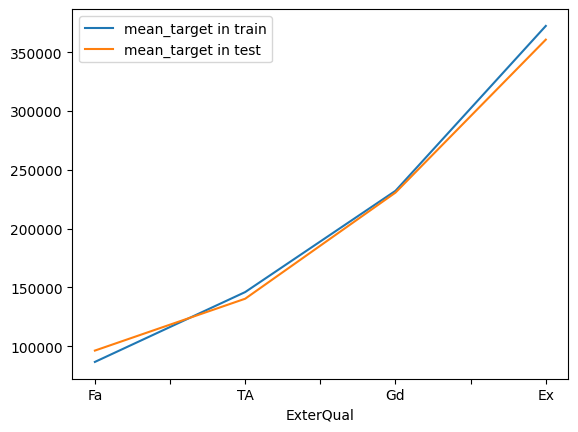
2.2.5.8. Monotonic target guided encoding#
The encoding is guided by the target, and create
monotonicrelationship between the variables and the target. (Đồng biến)Can be used on numerical variables after discretisation (convert to discrete)
Need to attention for handling rare labels
Note: Monotonic does not mean strictly linear. Monotonic means that it increases constantly, or it decreases constantly.
Need to explore original relationship between categorical variables and target by the mean value of target in each label via trainset and testset
1. Advantages
Straightforward to implement
Does not expand the feature space
Capture information within the category, therefore creating more predictive features
Creates monotonic relationship between categories and target, Create features suitable for linear models
1. Disadvantages
May lead to over-fitting
Difficult to implement together with cross-validation with current libraries
# function to explore monotonic relationship between target and categorical variable by train and testset
# With ordered label in trainset, we test the monotonic relationship in testset. If it was remained, that show there is a monotonic relationship
def check_monotonic(var, X_train, X_test, y_train, y_test):
    train = y_train.groupby(X_train[var]).mean().rename('mean_target in train')
    test = y_test.groupby(X_test[var]).mean().rename('mean_target in test')
    return pd.concat([train, test], axis = 1).sort_values('mean_target in train').interpolate().plot()

check_monotonic('ExterQual', X_train, X_test, y_train, y_test)
<AxesSubplot: xlabel='ExterQual'>
2.2.5.8.1. Ordered ordinal encoding#
Calculate the mean of target values for each label of variable, then assign numbers following the mean of target value from 0 (for highest mean) to k-1 (for smallest mean), with k is the number of distinct values of variable
Useful for
linearornon-linearmodel
# for encoding with feature-engine
from feature_engine.encoding import OrdinalEncoder

ordinal_enc = OrdinalEncoder(
    # NOTE that we indicate ordered in the encoding_method, otherwise it assings numbers arbitrarily
    encoding_method="ordered",
    variables=["Neighborhood", "ExterQual"],
)

ordinal_enc.fit(X_train, y_train)

# in the encoder dict we can observe each of the top categories selected for each of the variables
ordinal_enc.encoder_dict_
{'Neighborhood': {'IDOTRR': 0,
  'BrDale': 1,
  'MeadowV': 2,
  'Edwards': 3,
  'BrkSide': 4,
  'OldTown': 5,
  'Sawyer': 6,
  'Blueste': 7,
  'SWISU': 8,
  'NPkVill': 9,
  'NAmes': 10,
  'Mitchel': 11,
  'SawyerW': 12,
  'Gilbert': 13,
  'NWAmes': 14,
  'Blmngtn': 15,
  'CollgCr': 16,
  'ClearCr': 17,
  'Crawfor': 18,
  'Somerst': 19,
  'Veenker': 20,
  'Timber': 21,
  'NridgHt': 22,
  'StoneBr': 23,
  'NoRidge': 24},
 'ExterQual': {'Fa': 0, 'TA': 1, 'Gd': 2, 'Ex': 3}}
2.2.5.8.2. Mean encoding#
Replacing the category by the average target value for that category.
IF 2 categories show the same mean of target, they will have replace by the same number, lead to loss of value between them
from feature_engine.encoding import MeanEncoder

mean_enc = MeanEncoder(variables=["Neighborhood", "ExterQual"], smoothing = 10)
from feature_engine.encoding import WoEEncoder

pr_enc = WoEEncoder(variables = ["Neighborhood", "ExterQual"])
2.2.5.8.3. Weight of evidence encoding#
For each category
iofX, replaceibyWoe = Ln( P(X=i|Y=1) / P(X=i|Y=0) )These encoding is suitable for
logistic Regression, where thetargetisbinarySpecific Advantages to
Weight of evidence:It orders the categories on a “logistic” scale which is natural for logistic regression
The transformed variables can then be compared because they are on the same scale. Therefore, it is possible to determine which one is more predictive.
from feature_engine.encoding import WoEEncoder

pr_enc = WoEEncoder(variables = ["Neighborhood", "ExterQual"])